- Economy in the short-run: two factor income-expenditure model

Содержание
- 2. Lecture objectives What is the essence of the Keynesian doctrine? How can economic crises be explained
- 3. John Maynard Keynes (1883-1946) Model explaining causes of crises and suggesting methods of counteracting them. „The
- 4. The Keynesian perspective Aggregate demand as the cause of crises Government intervention as the remedy for
- 5. Model assumptions Two factor analysis: the only types of economic subjects are domestic households and firms
- 6. Circular flow in the model
- 7. The essence of aggregate demand Aggregate demand (AD): sum of expenditures for various goods and services
- 8. Consumption component of AD Two things concerning „C” must be noted: it is directly dependent on
- 9. Marginal propensity to consume Marginal propensity to consume (MPC): the fraction of the additional current income
- 10. Autonomous consumption Autonomous consumption (CA): the part of consumption that is not financed by current income
- 11. Consumption function Notice that MPC and CA are key variables in consumption function formula: 1) MPC
- 12. Technical note Changes in nouseholds’ current income result in shifts along the consumpion line. Changes in
- 13. Saving Saving means unconsumed income. Y = C + S C = MPC×Y + CA S
- 14. Saving function Notice that saving function is the mirror reflection of the consumption function formula: 1)
- 15. Investment component of AD Special status in the Keynesian doctrine Outstanding variability Independent of the current
- 16. Investment function
- 17. Aggregate demand: recollection Aggregate demand: the sum of households’ and firms’ expenditures (for consumption and investments,
- 18. Aggregate demand function
- 19. 45 degrees line At any point on the 45° line the distance to the horizontal axis
- 20. Check point: the meaning of „Y” So far the letter „Y” was using to denote „income”.
- 21. Keynesian cross Plotting AD and 45 degrees lines on the same chart allows you to study
- 22. Equilibrium & equilibrium output Equilibrium output (YE): the level of GDP at which the aggregate demand
- 23. Short-run equilibrium in the market for goods and services
- 24. Equilibrium: numerical example (static analysis) C = 50 + 0,7×Y S = – 50 + 0,3×Y
- 25. Equilibrium: two approaches First approach: AD = Y 450 + 0,7×Y = Y YE = 1500
- 26. Disequilibrium: shortage (insufficient production) STATUS Assume that Y = 1200 Then AD = 450 + 840
- 27. Disequilibrium: surplus (excess production) STATUS Assume that Y = 1800 Then AD = 450 + 1260
- 28. Beware of the misunderstanding! At the short-run disequilibrium: Splanned ≠ Iplanned Sactual = Iactual
- 29. Equilibrium: numerical example (dynamic analysis) Assume that: C = 50 + 0,7×Y I = 400 →
- 30. Investment multiplier Investment multiplier: a measure that informs how many times the change in the equilibrium
- 31. Investment multiplier and economic cycles Higher multiplier >>> more volatile GDP Lower multiplier >>> less volatile
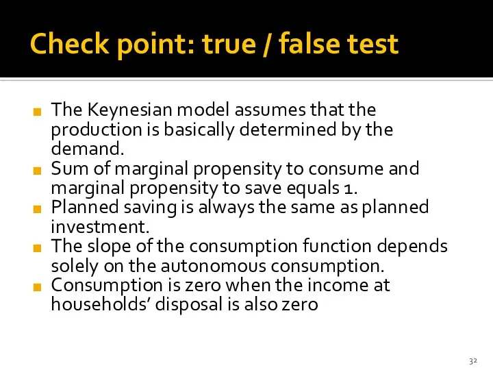
- 32. Check point: true / false test The Keynesian model assumes that the production is basically determined
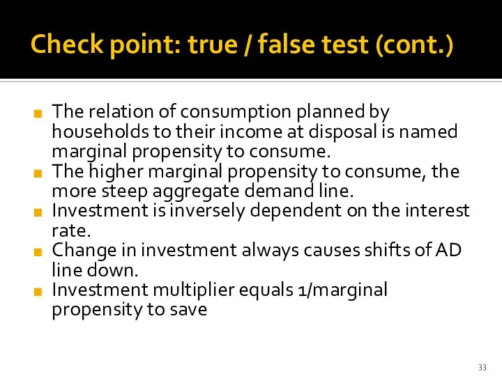
- 33. Check point: true / false test (cont.) The relation of consumption planned by households to their
- 34. Test your understanding: matching
- 35. Lecture objectives What is the essence of the Keynesian doctrine? How can economic crises be explained
- 37. Скачать презентацию
Lecture objectives
What is the essence of the Keynesian doctrine?
How can economic
Lecture objectives
What is the essence of the Keynesian doctrine?
How can economic

John Maynard Keynes
(1883-1946)
Model explaining causes of crises and suggesting methods
John Maynard Keynes
(1883-1946)
Model explaining causes of crises and suggesting methods
The Keynesian perspective
Aggregate demand as the cause of crises
Government intervention as
The Keynesian perspective
Aggregate demand as the cause of crises
Government intervention as

Model assumptions
Two factor analysis: the only types of economic subjects are
Model assumptions
Two factor analysis: the only types of economic subjects are

Circular flow in the model
Circular flow in the model
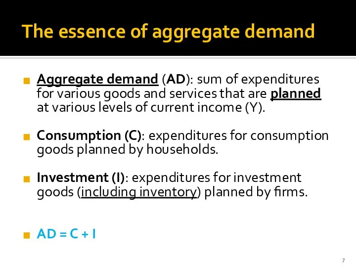
The essence of aggregate demand
Aggregate demand (AD): sum of expenditures for
The essence of aggregate demand
Aggregate demand (AD): sum of expenditures for
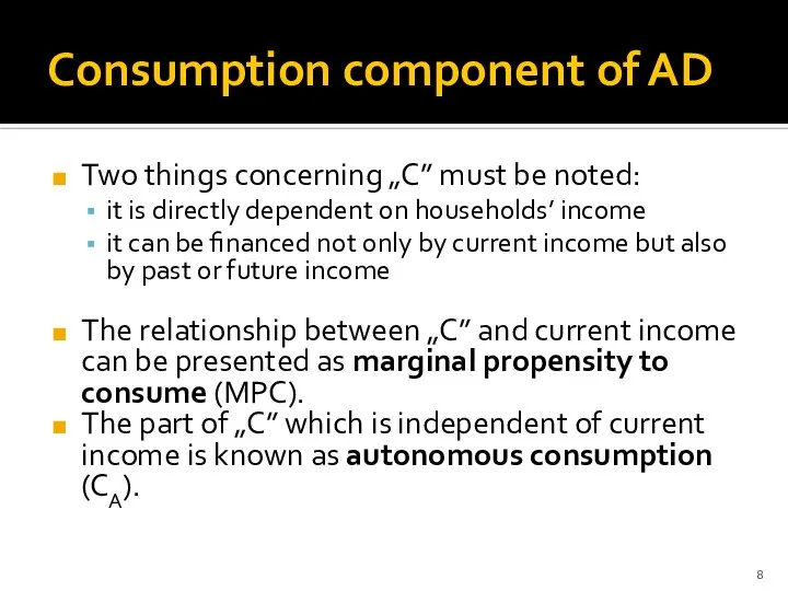
Consumption component of AD
Two things concerning „C” must be noted:
it is
Consumption component of AD
Two things concerning „C” must be noted:
it is
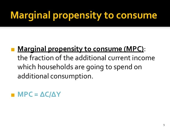
Marginal propensity to consume
Marginal propensity to consume (MPC):
the fraction of
Marginal propensity to consume
Marginal propensity to consume (MPC):
the fraction of
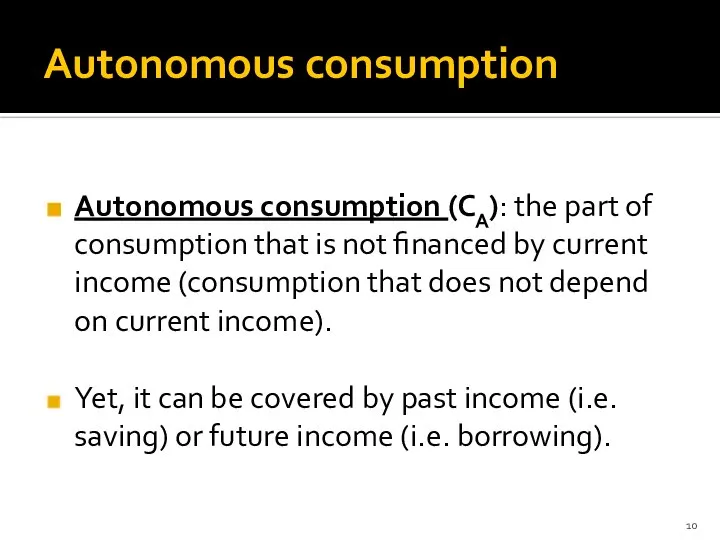
Autonomous consumption
Autonomous consumption (CA): the part of consumption that is not
Autonomous consumption
Autonomous consumption (CA): the part of consumption that is not
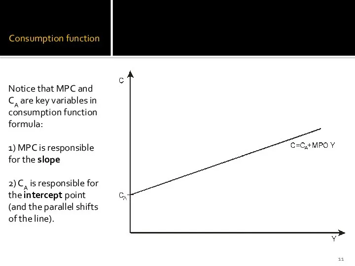
Consumption function
Notice that MPC and CA are key variables in consumption
Consumption function
Notice that MPC and CA are key variables in consumption
Technical note
Changes in nouseholds’ current income result in shifts along the
Technical note
Changes in nouseholds’ current income result in shifts along the
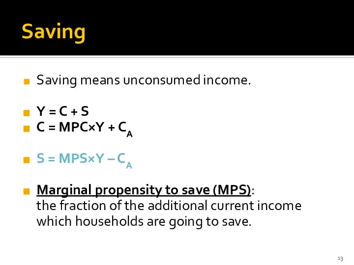
Saving
Saving means unconsumed income.
Y = C + S
C = MPC×Y +
Saving
Saving means unconsumed income.
Y = C + S
C = MPC×Y +
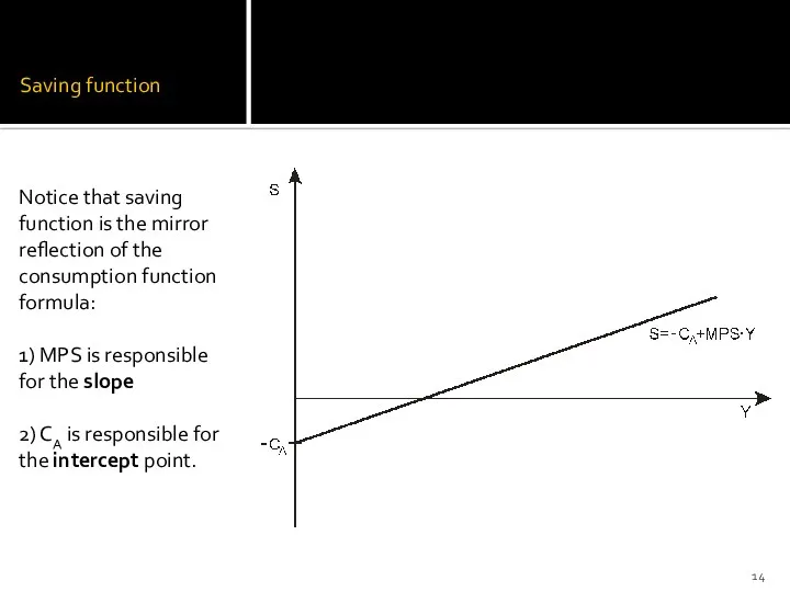
Saving function
Notice that saving function is the mirror reflection of the
Saving function
Notice that saving function is the mirror reflection of the
Investment component of AD
Special status in the Keynesian doctrine
Outstanding variability
Independent of
Investment component of AD
Special status in the Keynesian doctrine
Outstanding variability
Independent of

Investment function
Investment function
Aggregate demand: recollection
Aggregate demand: the sum of households’ and firms’ expenditures
Aggregate demand: recollection
Aggregate demand: the sum of households’ and firms’ expenditures
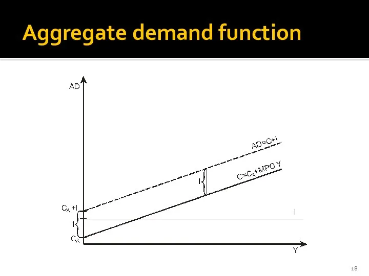
Aggregate demand function
Aggregate demand function

45 degrees line
At any point on the 45° line the distance
45 degrees line
At any point on the 45° line the distance
Check point: the meaning of „Y”
So far the letter „Y” was
Check point: the meaning of „Y”
So far the letter „Y” was

Keynesian cross
Plotting AD and 45 degrees lines on the same chart
Keynesian cross
Plotting AD and 45 degrees lines on the same chart
Equilibrium & equilibrium output
Equilibrium output (YE): the level of GDP at
Equilibrium & equilibrium output
Equilibrium output (YE): the level of GDP at

Short-run equilibrium in the market for goods and services
Short-run equilibrium in the market for goods and services
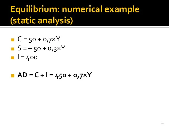
Equilibrium: numerical example (static analysis)
C = 50 + 0,7×Y
S = –
Equilibrium: numerical example (static analysis)
C = 50 + 0,7×Y
S = –
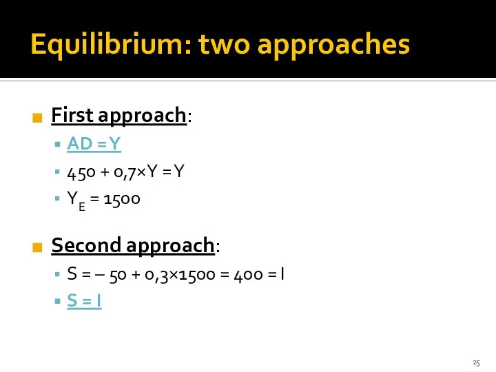
Equilibrium: two approaches
First approach:
AD = Y
450 + 0,7×Y = Y
YE =
Equilibrium: two approaches
First approach:
AD = Y
450 + 0,7×Y = Y
YE =

Disequilibrium: shortage (insufficient production)
STATUS
Assume that
Y = 1200
Then AD = 450
Disequilibrium: shortage (insufficient production)
STATUS
Assume that
Y = 1200
Then AD = 450

Disequilibrium: surplus (excess production)
STATUS
Assume that
Y = 1800
Then AD = 450
Disequilibrium: surplus (excess production)
STATUS
Assume that
Y = 1800
Then AD = 450
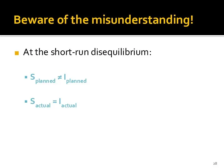
Beware of the misunderstanding!
At the short-run disequilibrium:
Splanned ≠ Iplanned
Sactual = Iactual
Beware of the misunderstanding!
At the short-run disequilibrium:
Splanned ≠ Iplanned
Sactual = Iactual

Equilibrium: numerical example (dynamic analysis)
Assume that:
C = 50 + 0,7×Y
I =
Equilibrium: numerical example (dynamic analysis)
Assume that:
C = 50 + 0,7×Y
I =

Investment multiplier
Investment multiplier: a measure that informs how many times the
Investment multiplier
Investment multiplier: a measure that informs how many times the

Investment multiplier and economic cycles
Higher multiplier >>> more volatile GDP
Lower multiplier
Investment multiplier and economic cycles
Higher multiplier >>> more volatile GDP
Lower multiplier
Check point: true / false test
The Keynesian model assumes that the
Check point: true / false test
The Keynesian model assumes that the
Check point: true / false test (cont.)
The relation of consumption planned
Check point: true / false test (cont.)
The relation of consumption planned

Test your understanding: matching
Test your understanding: matching

Lecture objectives
What is the essence of the Keynesian doctrine?
How can economic
Lecture objectives
What is the essence of the Keynesian doctrine?
How can economic
 Міжнародний проект з транскордонного співробітництва у Вінницькій області
 Глобальные проблемы человечества и пути их решения
 Сегментация рынка труда. Рынок труда отдельных групп населения
 Проблемы и перспективы Томска как центра инноваций и новых технологий
 Экономика. Основные участники экономического процесса
 Общая характеристика Восточного макрорегиона
 Теория потребительского поведения
 Специфика процесса урбанизации в XXI веке. (Тема 1)
 Виробництво та продукт економічної діяльності. Виробничі технології. Особливість сучасних технологій
 Основной капитал и основные фонды предприятия
 Теория организации рынков
 Общее понятие предпринимательства
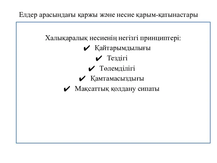 Елдер арасындағы қаржы және несие қарым-қатынастары
 Вводная лекция. Высшая школа экономики
 Презентация Таможенные льготы в Таможенном союзе
 Дүние жүзілік сауда ұйымы (ДСҰ)
 Теоретические основы организации туристской отрасли
 Международные валютные отношения и валютный рынок. (Темы 1-2) Валюта как ключевая категория международных валютных отношений
 Сущность, предмет и объект изучения экономической статистики
 Економіка СРСР у 70-х роках
 Сказка о том как провести анализ спроса
 Типы экономических систем (тест)
 Интернациональная система качественного развития РФ
 Повышение эффективности использования оборотных средств предприятия
 Трансформационный кризис в России в 1990-х гг.: общая характеристика
 Шведская модель рыночной экономики
 Элементы теории игр
 Презентация КОРРУПЦИЯ