- Macroeconomics. Introduction

Содержание
- 2. Introduction Structure of course Chapter 1 The date and methods of macroeconomics Chapter 2-4 The National
- 3. Introduction Structure of course Chapter 5 The Determination of Output, Income, Expenditure and a Model of
- 4. Introduction Structure of course Chapter 7 Labour Market, Employment, Unemployment Chapter 8 Economic Fluctuations
- 5. Introduction Structure of course Chapter 9 The Keynsian Model of Short-Run Equilibrium Chapter 10 Aggregate Supply
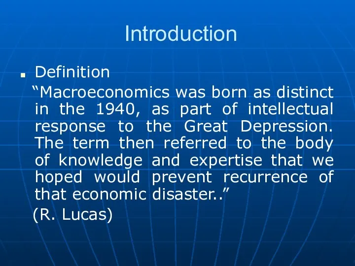
- 6. Introduction Definition “Macroeconomics was born as distinct in the 1940, as part of intellectual response to
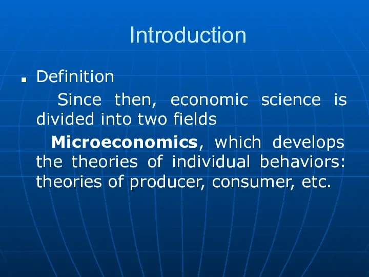
- 7. Introduction Definition Since then, economic science is divided into two fields Microeconomics, which develops the theories
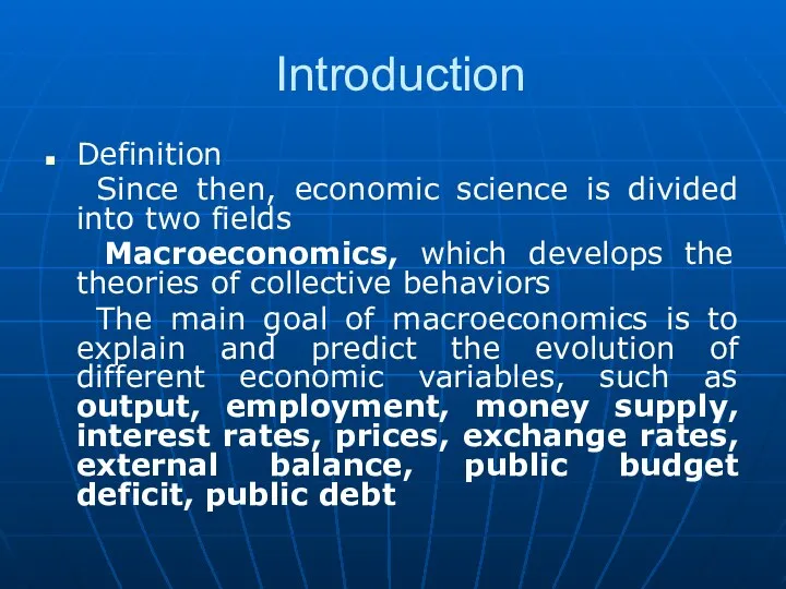
- 8. Introduction Definition Since then, economic science is divided into two fields Macroeconomics, which develops the theories
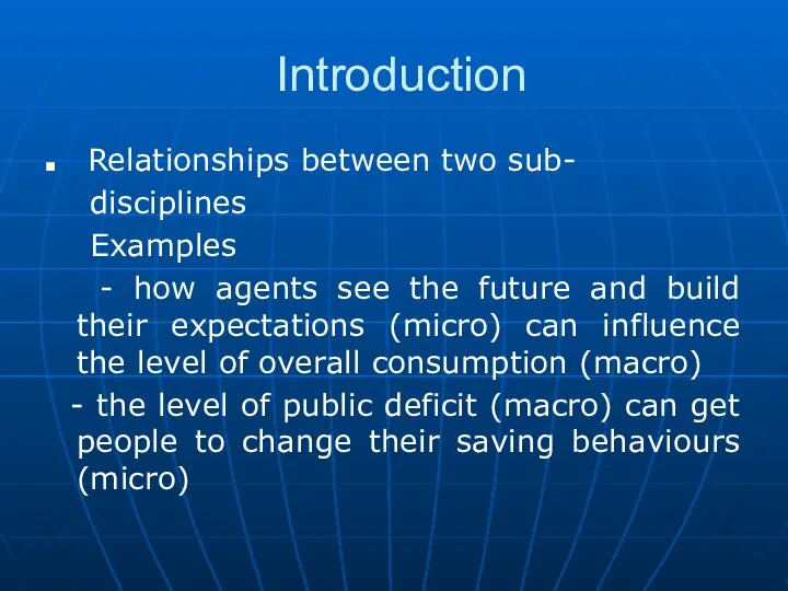
- 9. Introduction Relationships between two sub- disciplines Examples - how agents see the future and build their
- 10. Introduction An overview of the macroeconomic theories Two main theories: - Classical theory gives a central
- 11. Introduction An overview of the macroeconomic theories Classical theory- economic policies are not helpful. Market can
- 12. Introduction An overview of the macroeconomic theories Keynesian theory – economic policies are useful because the
- 13. Introduction An overview of the macroeconomic theories Classical theory- Hypothesis of flexible prices, macroeconomic theories may
- 14. Introduction An overview of the macroeconomic theories Keynsian theory helps to explain the short-run fluctuations in
- 15. Introduction The Empirical Aspects of the Macro-economics The macro circuit means a non-theoretical representation of economic
- 16. Introduction The Empirical Aspects of the Macro-economics The output is the value, expressed in money. This
- 17. Introduction The Empirical Aspects of the Macro-economics Expenditure means the money value of purchases of goods
- 18. Introduction The Empirical Aspects of the Macro-economics Macroeconomic subjects
- 19. Introduction The Empirical Aspects of the Macro-economics OUTPUT=INCOME=EXPENDITURE
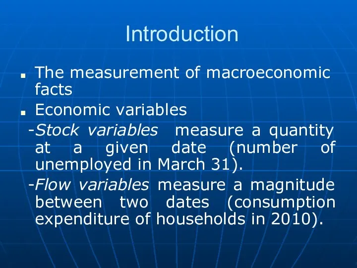
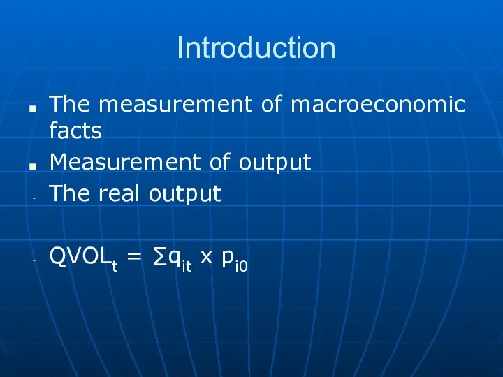
- 20. Introduction The measurement of macroeconomic facts Economic variables -Stock variables measure a quantity at a given
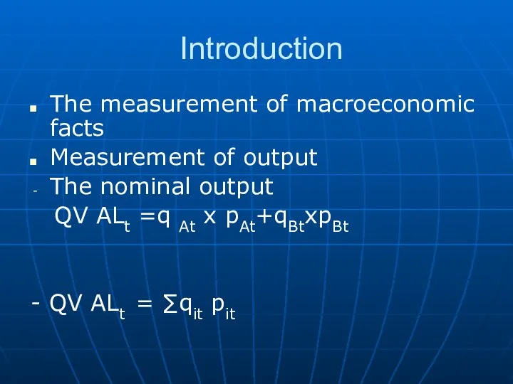
- 21. Introduction The measurement of macroeconomic facts Measurement of output The nominal output QV ALt =q At
- 22. Introduction The measurement of macroeconomic facts Measurement of output The real output QVOLt = ∑qit x
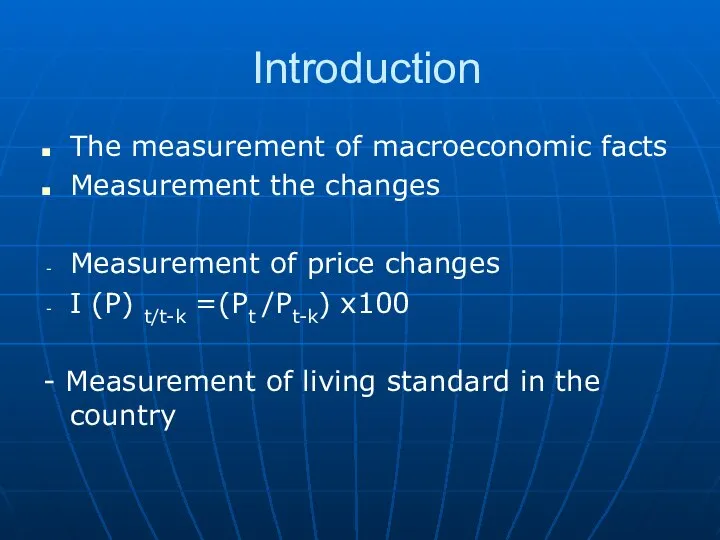
- 23. Introduction The measurement of macroeconomic facts Measurement the changes Measurement of price changes I (P) t/t-k
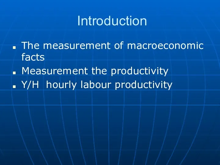
- 24. Introduction The measurement of macroeconomic facts Measurement the productivity Y/H hourly labour productivity
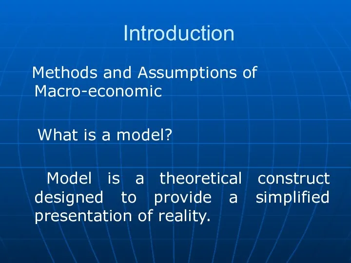
- 25. Introduction Methods and Assumptions of Macro-economic What is a model? Model is a theoretical construct designed
- 26. Introduction Methods and Assumptions of Macro-economic What is a model? Example- a model of economic equilibrium
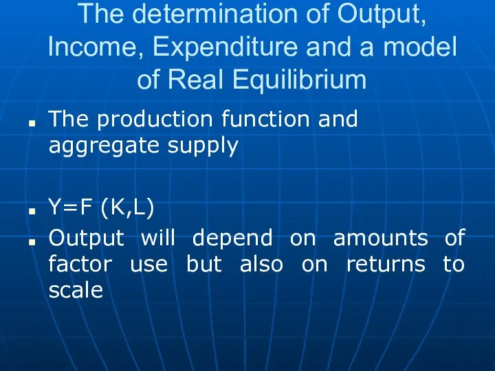
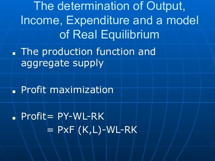
- 27. The determination of Output, Income, Expenditure and a model of Real Equilibrium The production function and
- 28. The determination of Output, Income, Expenditure and a model of Real Equilibrium The production function and
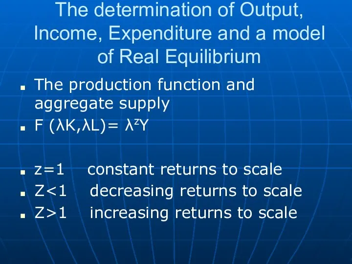
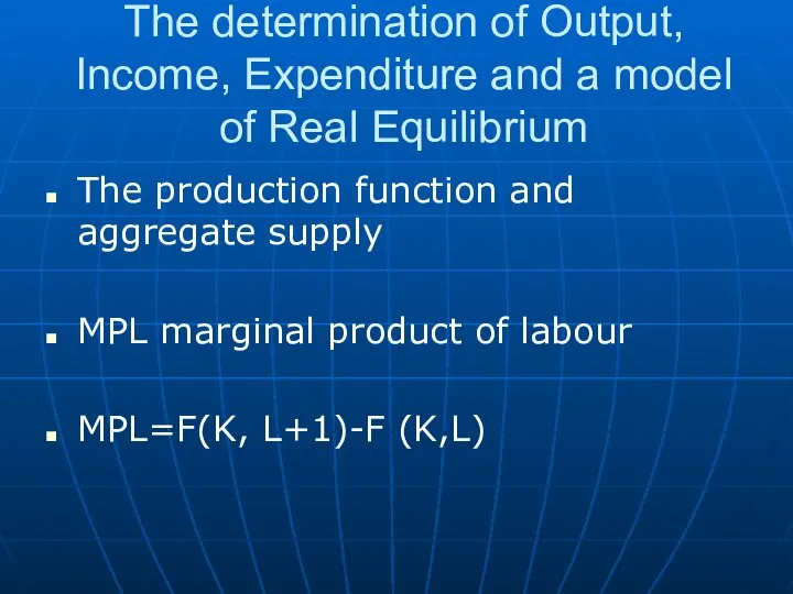
- 29. The determination of Output, Income, Expenditure and a model of Real Equilibrium The production function and
- 30. The determination of Output, Income, Expenditure and a model of Real Equilibrium The production function and
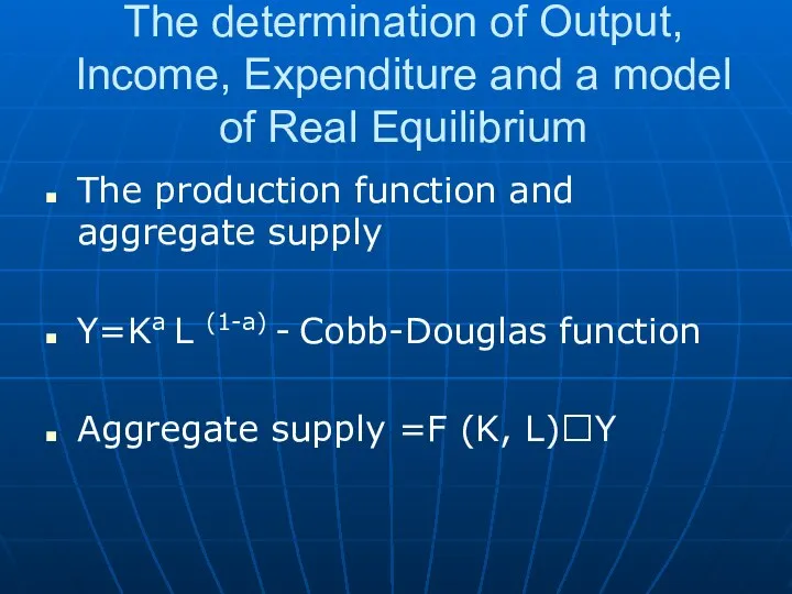
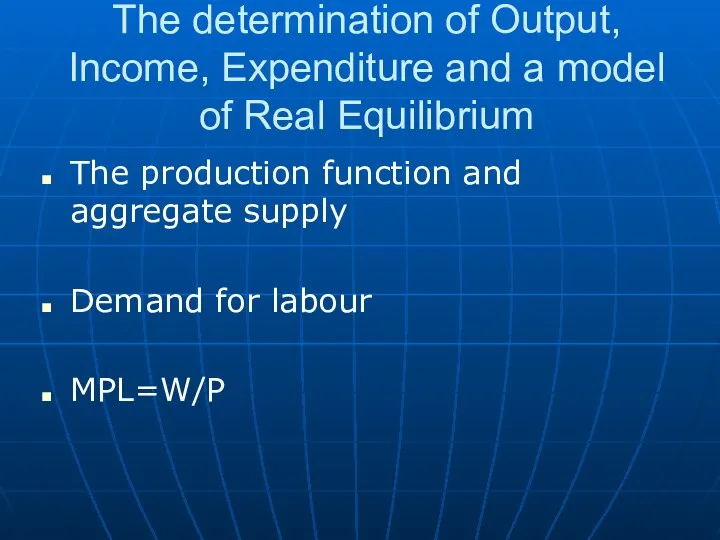
- 31. The determination of Output, Income, Expenditure and a model of Real Equilibrium The production function and
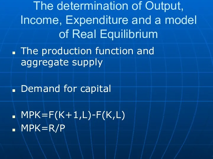
- 32. The determination of Output, Income, Expenditure and a model of Real Equilibrium The production function and
- 33. The determination of Output, Income, Expenditure and a model of Real Equilibrium The production function and
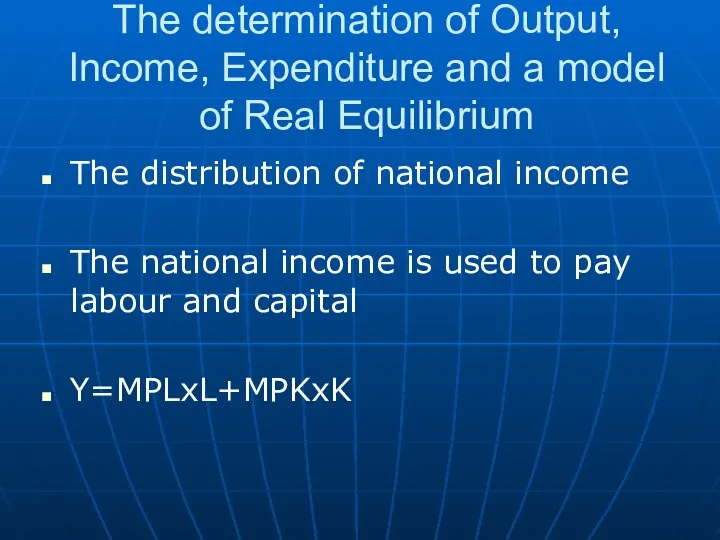
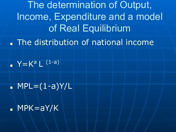
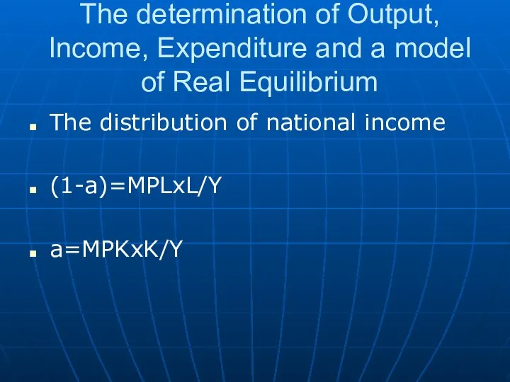
- 34. The determination of Output, Income, Expenditure and a model of Real Equilibrium The distribution of national
- 35. The determination of Output, Income, Expenditure and a model of Real Equilibrium The distribution of national
- 36. The determination of Output, Income, Expenditure and a model of Real Equilibrium The distribution of national
- 37. The determination of Output, Income, Expenditure and a model of Real Equilibrium The distribution of national
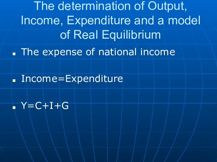
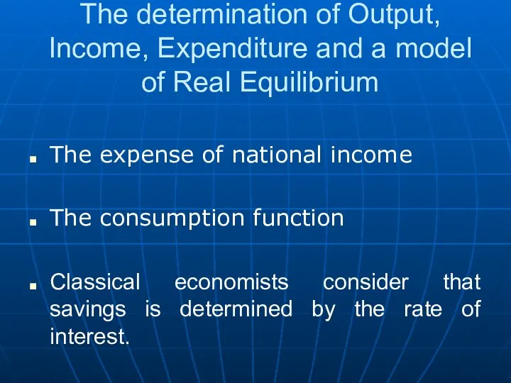
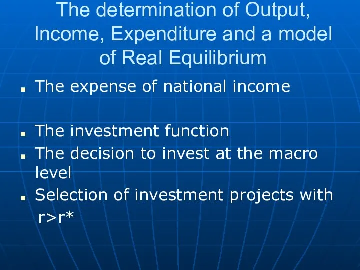
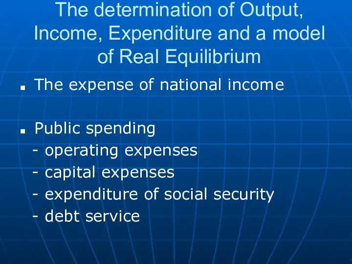
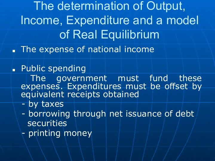
- 38. The determination of Output, Income, Expenditure and a model of Real Equilibrium The expense of national
- 39. The determination of Output, Income, Expenditure and a model of Real Equilibrium The expense of national
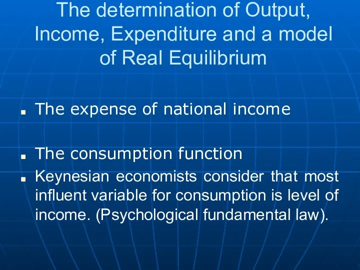
- 40. The determination of Output, Income, Expenditure and a model of Real Equilibrium The expense of national
- 41. The determination of Output, Income, Expenditure and a model of Real Equilibrium The expense of national
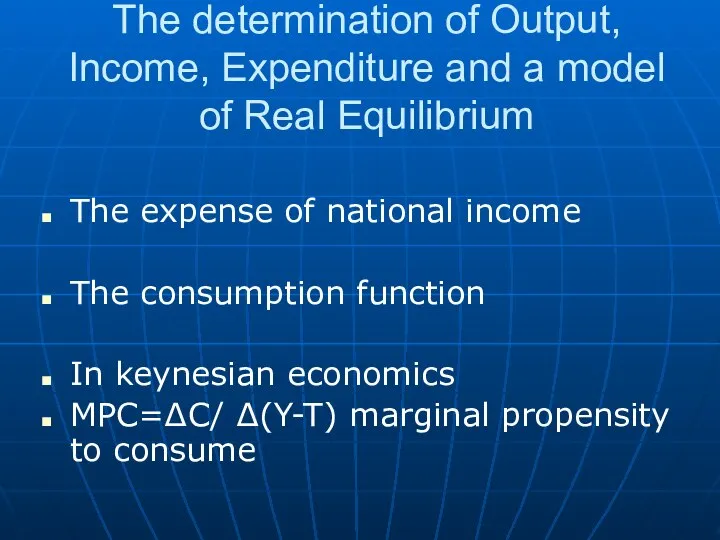
- 42. The determination of Output, Income, Expenditure and a model of Real Equilibrium The expense of national
- 43. The determination of Output, Income, Expenditure and a model of Real Equilibrium The expense of national
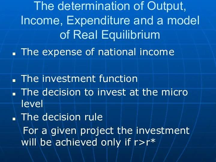
- 44. The determination of Output, Income, Expenditure and a model of Real Equilibrium The expense of national
- 45. The determination of Output, Income, Expenditure and a model of Real Equilibrium The expense of national
- 46. The determination of Output, Income, Expenditure and a model of Real Equilibrium The expense of national
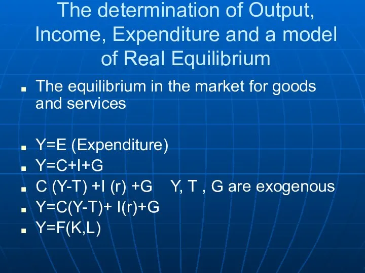
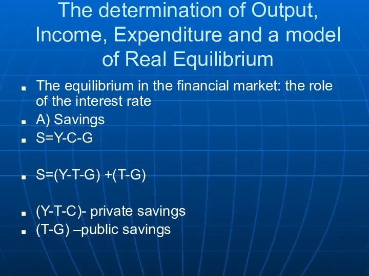
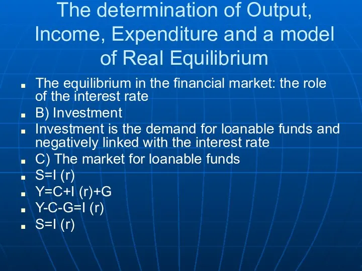
- 47. The determination of Output, Income, Expenditure and a model of Real Equilibrium The equilibrium in the
- 48. The determination of Output, Income, Expenditure and a model of Real Equilibrium The equilibrium in the
- 49. The determination of Output, Income, Expenditure and a model of Real Equilibrium The equilibrium in the
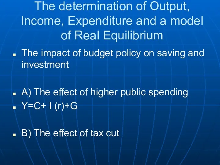
- 50. The determination of Output, Income, Expenditure and a model of Real Equilibrium The impact of budget
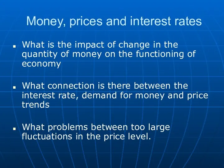
- 51. Money, prices and interest rates What is the impact of change in the quantity of money
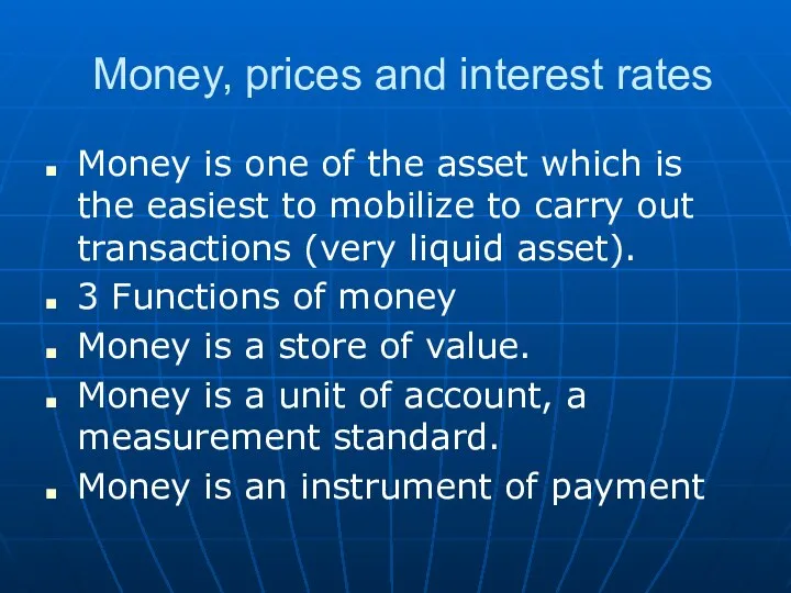
- 52. Money, prices and interest rates Money is one of the asset which is the easiest to
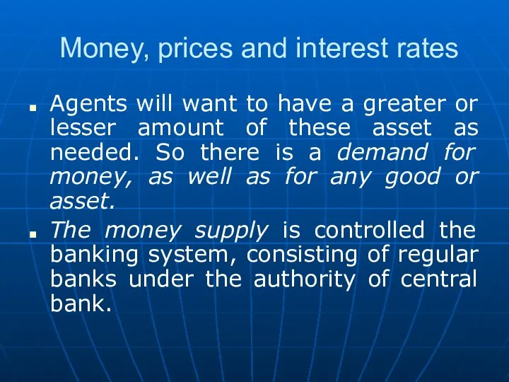
- 53. Money, prices and interest rates Agents will want to have a greater or lesser amount of
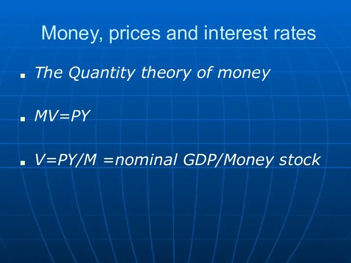
- 54. Money, prices and interest rates The Quantity theory of money MV=PY V=PY/M =nominal GDP/Money stock
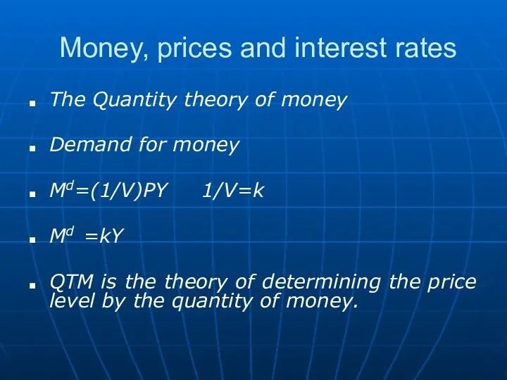
- 55. Money, prices and interest rates The Quantity theory of money Demand for money Md=(1/V)PY 1/V=k Md
- 56. Money, prices and interest Rates The Interest Rate, the demand for money and Inflation The nominal
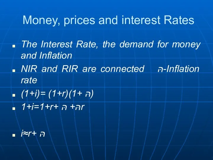
- 57. Money, prices and interest Rates The Interest Rate, the demand for money and Inflation NIR and
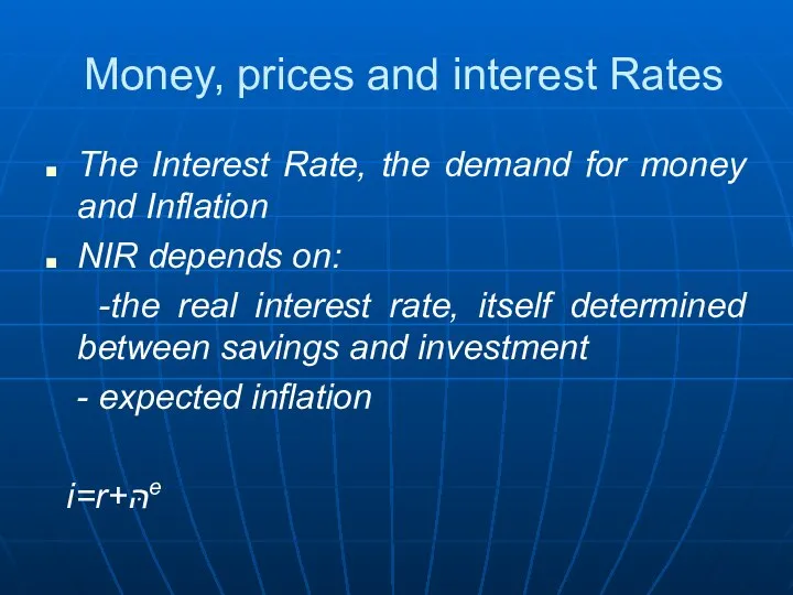
- 58. Money, prices and interest Rates The Interest Rate, the demand for money and Inflation NIR depends
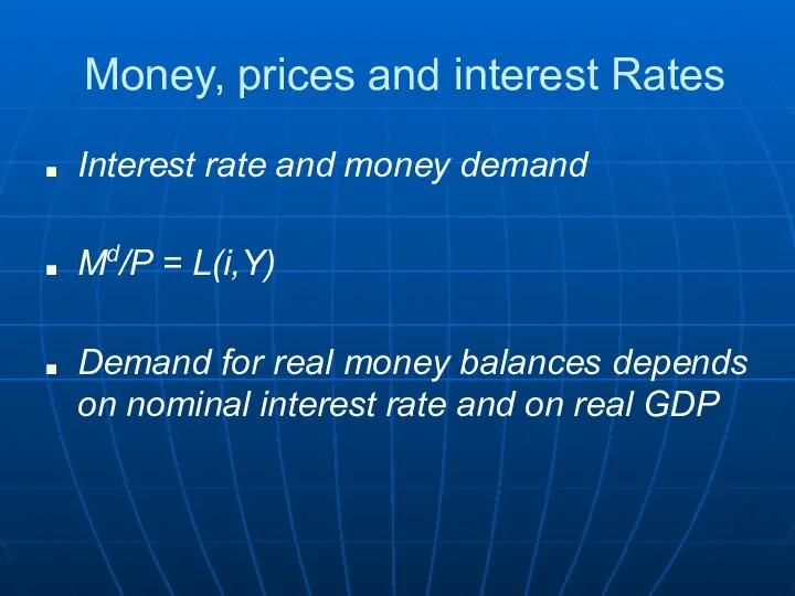
- 59. Money, prices and interest Rates Interest rate and money demand Md/P = L(i,Y) Demand for real
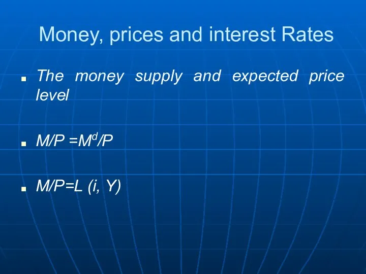
- 60. Money, prices and interest Rates The money supply and expected price level M/P =Md/P M/P=L (i,
- 61. Money, prices and interest rates The money supply and expected price level M/P=L (r+ הּe, Y
- 62. Money, prices and interest rates The Problems with Too Large Fluctuation in Price Level Inflation is
- 63. Money, prices and interest rates The Problems with Too Large Fluctuation in Price Level Deflation is
- 64. Labour market, employment, unemployment Labour demand comes from com-panies that want to produce. Labour supply comes
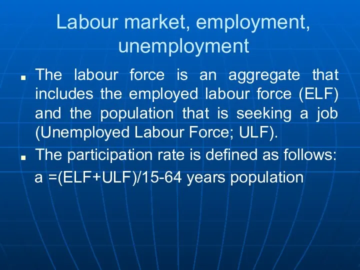
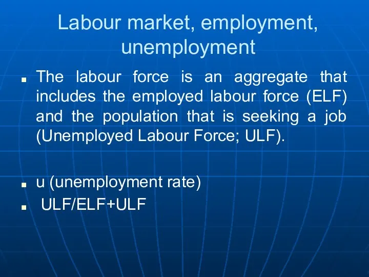
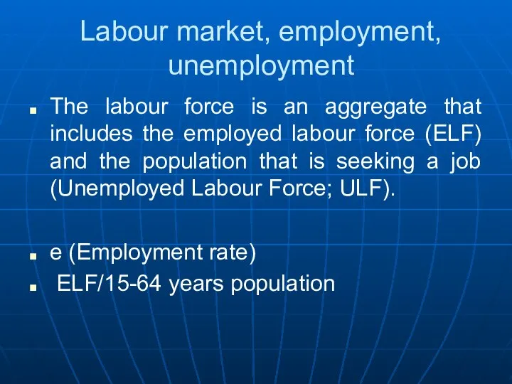
- 65. Labour market, employment, unemployment The labour force is an aggregate that includes the employed labour force
- 66. Labour market, employment, unemployment The labour force is an aggregate that includes the employed labour force
- 67. Labour market, employment, unemployment The labour force is an aggregate that includes the employed labour force
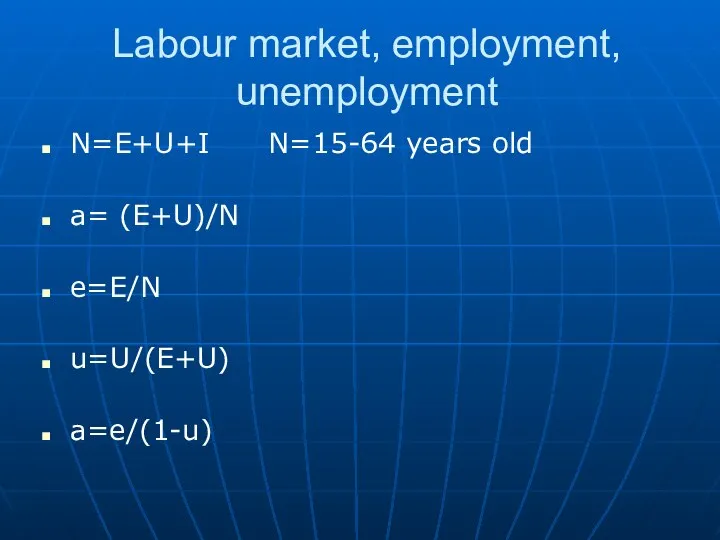
- 68. Labour market, employment, unemployment N=E+U+I N=15-64 years old a= (E+U)/N e=E/N u=U/(E+U) a=e/(1-u)
- 69. Labour market, employment, unemployment Share of long length unemployed (those unemployed for one year and more)
- 70. Labour market, employment, unemployment The flow of workers It is the number of people who, over
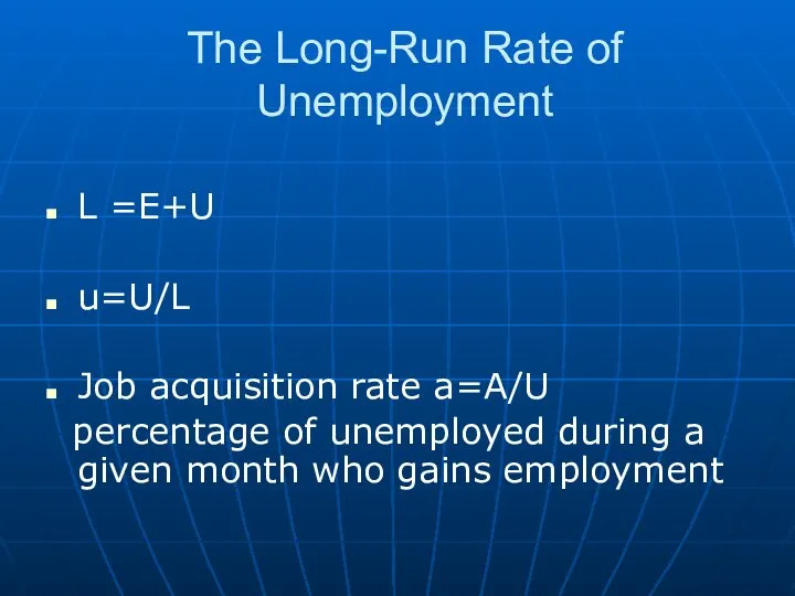
- 71. The Long-Run Rate of Unemployment L =E+U u=U/L Job acquisition rate a=A/U percentage of unemployed during
- 72. The Long-Run Rate of Unemployment L =E+U u=U/L Job loss rate p=P/U percentage of employees who
- 73. The Long-Run Rate of Unemployment Natural rate of unemployment=long-run rate of unemployment A=P
- 74. Economic fluctuations The economy is experiencing fluctuations that result in variations in the level of output
- 75. Economic fluctuations Acceleration phases (economic boom) Contraction phase (economic recession)
- 76. Economic fluctuations Changes in output and unemployment When the economy is bad, cyclical unemployment, adds to
- 77. Economic fluctuations Changes in output and unemployment When the economy is bad, cyclical unemployment, adds to
- 78. Economic fluctuations Changes in output and unemployment When the economy is bad, cyclical unemployment, adds to
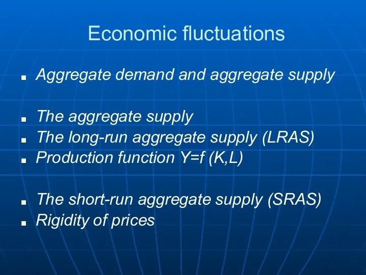
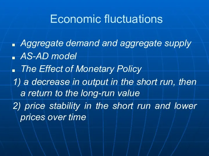
- 79. Economic fluctuations Aggregate demand and aggregate supply The aggregate demand is deduced from the quantity aquation
- 80. Economic fluctuations Aggregate demand and aggregate supply The aggregate supply The long-run aggregate supply (LRAS) Production
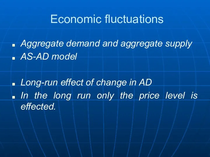
- 81. Economic fluctuations Aggregate demand and aggregate supply AS-AD model Long-run effect of change in AD In
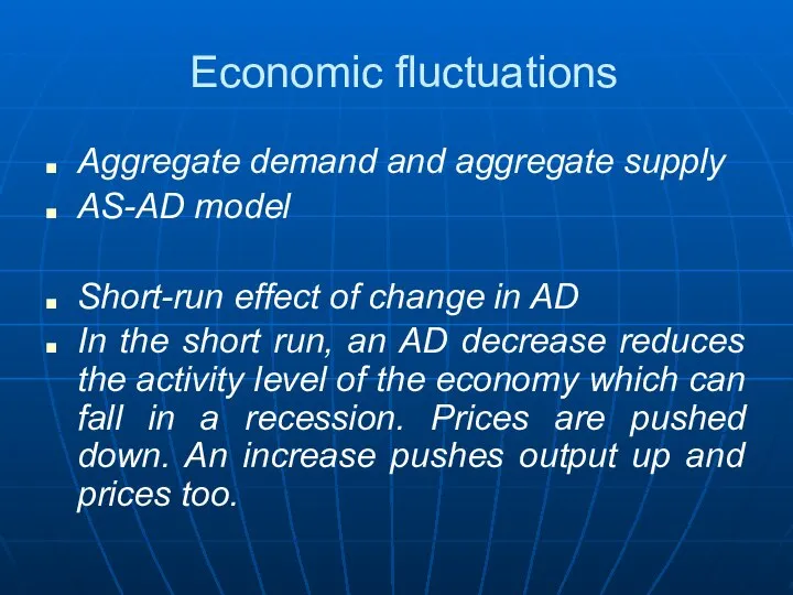
- 82. Economic fluctuations Aggregate demand and aggregate supply AS-AD model Short-run effect of change in AD In
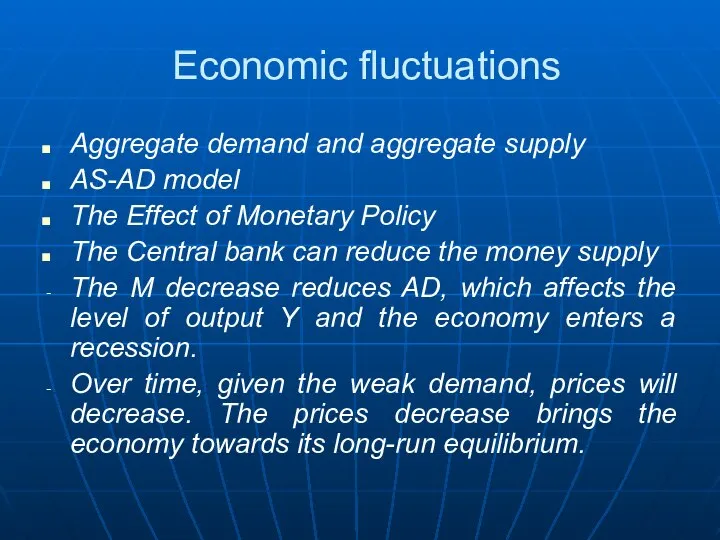
- 83. Economic fluctuations Aggregate demand and aggregate supply AS-AD model The Effect of Monetary Policy The Central
- 84. Economic fluctuations Aggregate demand and aggregate supply AS-AD model The Effect of Monetary Policy 1) a
- 85. Economic fluctuations Aggregate demand and aggregate supply AS-AD model The Effect of Monetary Policy 1) a
- 86. Economic fluctuations Aggregate demand and aggregate supply AS-AD model The Effect of Monetary Policy 1) a
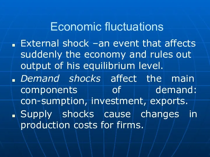
- 87. Economic fluctuations External shock –an event that affects suddenly the economy and rules out output of
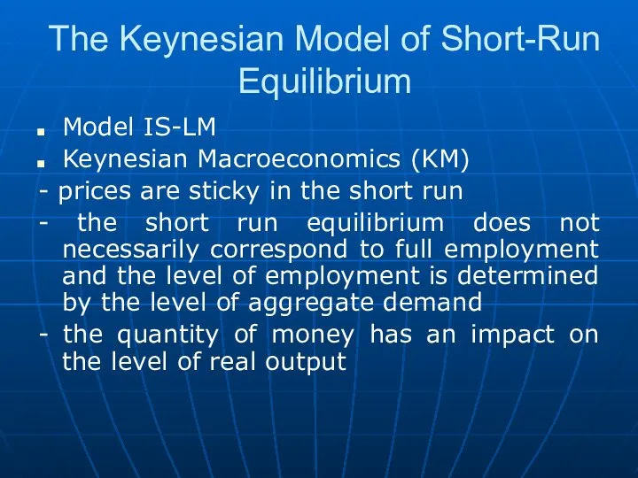
- 88. The Keynesian Model of Short-Run Equilibrium Model IS-LM Keynesian Macroeconomics (KM) - prices are sticky in
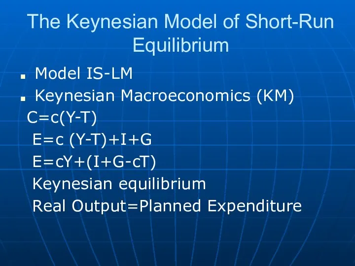
- 89. The Keynesian Model of Short-Run Equilibrium Model IS-LM Keynesian Macroeconomics (KM) C=c(Y-T) E=c (Y-T)+I+G E=cY+(I+G-cT) Keynesian
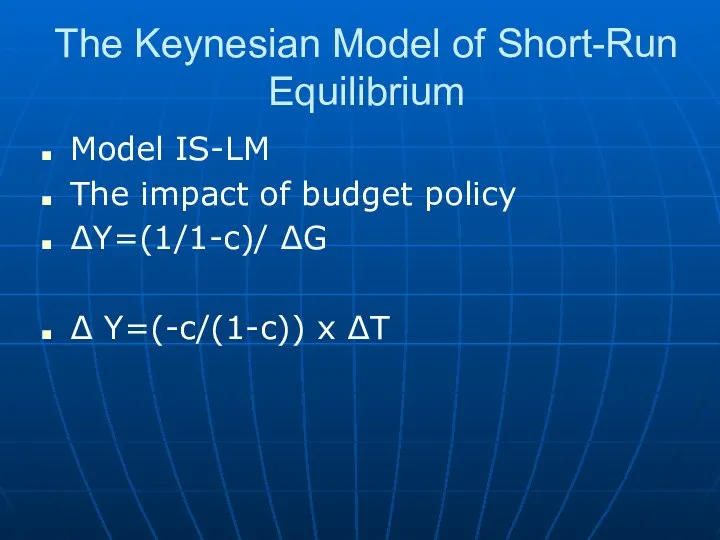
- 90. The Keynesian Model of Short-Run Equilibrium Model IS-LM The impact of budget policy ∆Y=(1/1-c)/ ∆G ∆
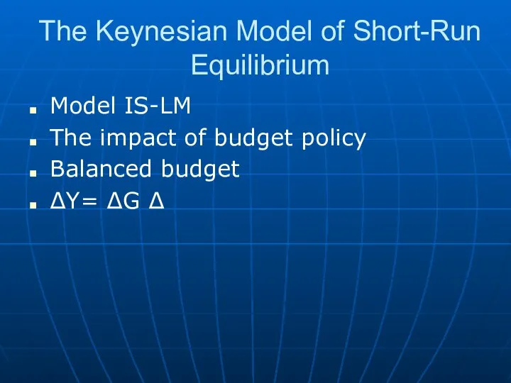
- 91. The Keynesian Model of Short-Run Equilibrium Model IS-LM The impact of budget policy Balanced budget ∆Y=
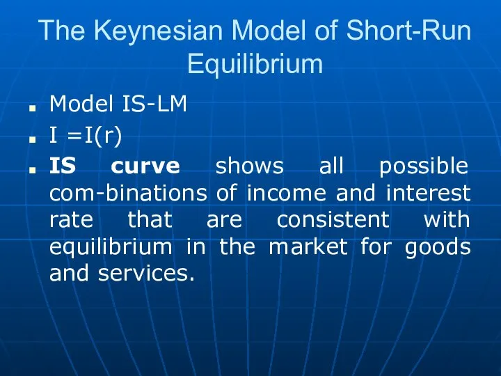
- 92. The Keynesian Model of Short-Run Equilibrium Model IS-LM I =I(r) IS curve shows all possible com-binations
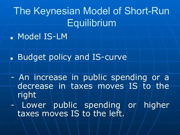
- 93. The Keynesian Model of Short-Run Equilibrium Model IS-LM Budget policy and IS-curve - An increase in
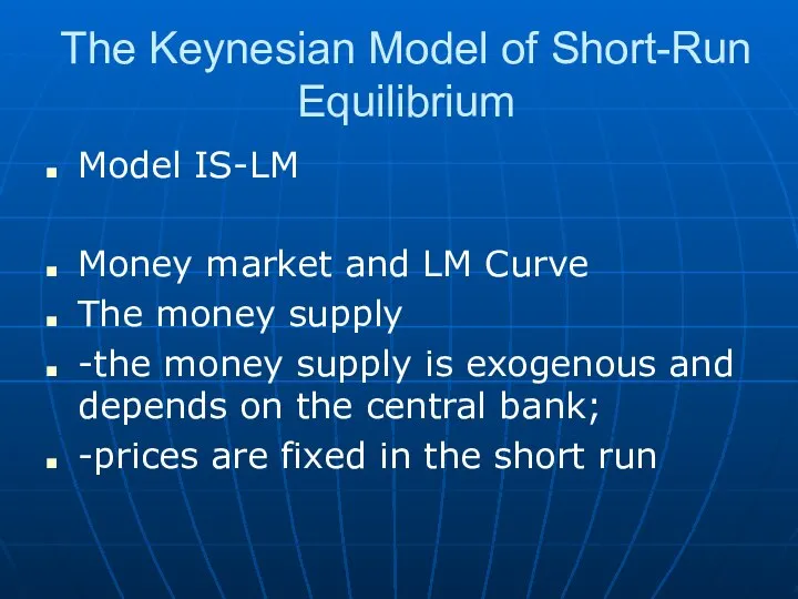
- 94. The Keynesian Model of Short-Run Equilibrium Model IS-LM Money market and LM Curve The money supply
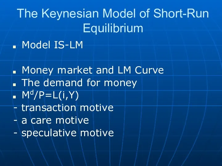
- 95. The Keynesian Model of Short-Run Equilibrium Model IS-LM Money market and LM Curve The demand for
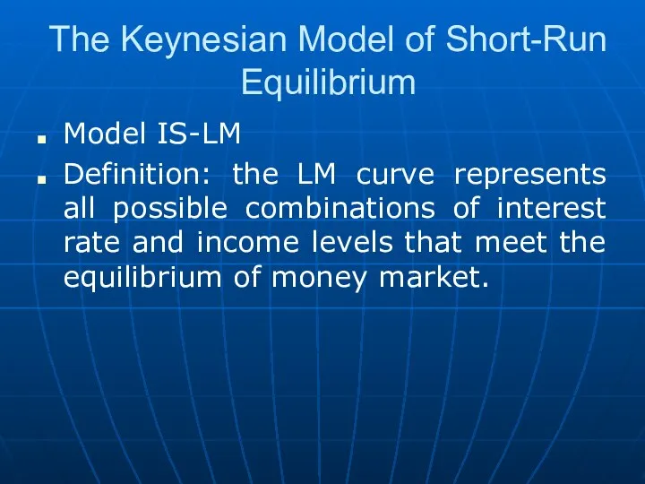
- 96. The Keynesian Model of Short-Run Equilibrium Model IS-LM Definition: the LM curve represents all possible combinations
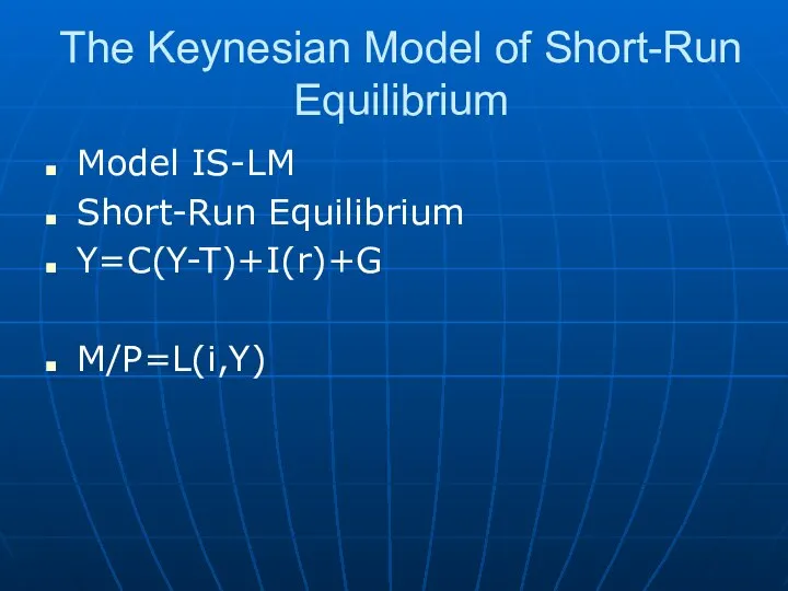
- 97. The Keynesian Model of Short-Run Equilibrium Model IS-LM Short-Run Equilibrium Y=C(Y-T)+I(r)+G M/P=L(i,Y)
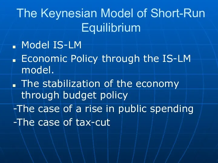
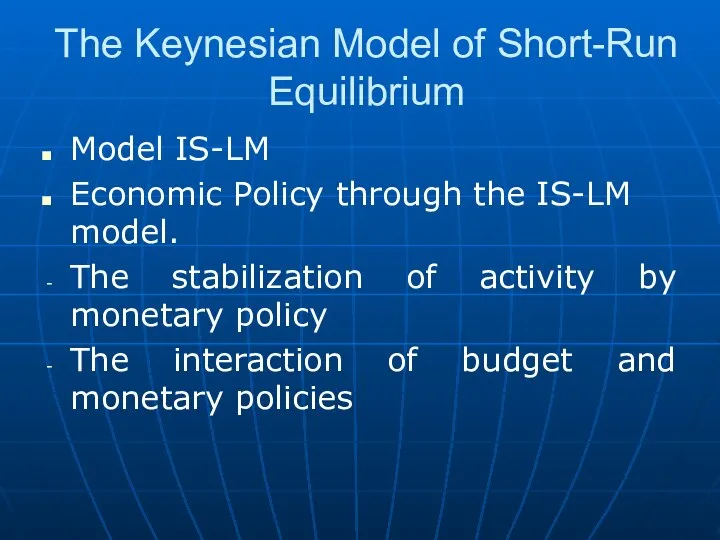
- 98. The Keynesian Model of Short-Run Equilibrium Model IS-LM Economic Policy through the IS-LM model. The stabilization
- 99. The Keynesian Model of Short-Run Equilibrium Model IS-LM Economic Policy through the IS-LM model. The stabilization
- 100. The Keynesian Model of Short-Run Equilibrium Model IS-LM IS-LM and aggregate demand IS-LM and deflation
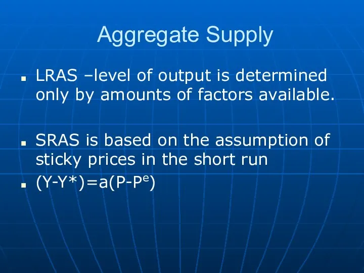
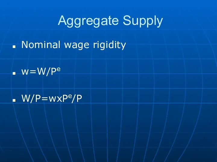
- 101. Aggregate Supply LRAS –level of output is determined only by amounts of factors available. SRAS is
- 102. Aggregate Supply Nominal wage rigidity w=W/Pe W/P=wxPe/P
- 104. Скачать презентацию
Introduction
Structure of course
Chapter 1 The date and methods of macroeconomics
Chapter
Introduction
Structure of course
Chapter 1 The date and methods of macroeconomics
Chapter
Introduction
Structure of course
Chapter 5 The Determination of Output, Income, Expenditure and
Introduction
Structure of course
Chapter 5 The Determination of Output, Income, Expenditure and
Introduction
Structure of course
Chapter 7 Labour Market, Employment, Unemployment
Chapter 8 Economic
Introduction
Structure of course
Chapter 7 Labour Market, Employment, Unemployment
Chapter 8 Economic
Introduction
Structure of course
Chapter 9 The Keynsian Model of
Short-Run Equilibrium
Introduction
Structure of course
Chapter 9 The Keynsian Model of
Short-Run Equilibrium
Introduction
Definition
“Macroeconomics was born as distinct in the 1940, as part
Introduction
Definition
“Macroeconomics was born as distinct in the 1940, as part
Introduction
Definition
Since then, economic science is divided into two fields
Introduction
Definition
Since then, economic science is divided into two fields
Introduction
Definition
Since then, economic science is divided into two fields
Introduction
Definition
Since then, economic science is divided into two fields
Introduction
Relationships between two sub-
disciplines
Examples
- how
Introduction
Relationships between two sub-
disciplines
Examples
- how
Introduction
An overview of the macroeconomic theories
Two main theories:
-
Introduction
An overview of the macroeconomic theories
Two main theories:
-
Introduction
An overview of the macroeconomic theories
Classical theory- economic policies are not
Introduction
An overview of the macroeconomic theories
Classical theory- economic policies are not
Introduction
An overview of the macroeconomic theories
Keynesian theory – economic policies are
Introduction
An overview of the macroeconomic theories
Keynesian theory – economic policies are
Introduction
An overview of the macroeconomic theories
Classical theory-
Hypothesis of flexible prices, macroeconomic
Introduction
An overview of the macroeconomic theories
Classical theory-
Hypothesis of flexible prices, macroeconomic
Introduction
An overview of the macroeconomic theories
Keynsian theory helps to explain the
Introduction
An overview of the macroeconomic theories
Keynsian theory helps to explain the
Introduction
The Empirical Aspects of the Macro-economics
The macro circuit means a non-theoretical
Introduction
The Empirical Aspects of the Macro-economics
The macro circuit means a non-theoretical
Introduction
The Empirical Aspects of the Macro-economics
The output is the value, expressed
Introduction
The Empirical Aspects of the Macro-economics
The output is the value, expressed
Introduction
The Empirical Aspects of the Macro-economics
Expenditure means the money value of
Introduction
The Empirical Aspects of the Macro-economics
Expenditure means the money value of
Introduction
The Empirical Aspects of the Macro-economics
Macroeconomic subjects
Introduction
The Empirical Aspects of the Macro-economics
Macroeconomic subjects
Introduction
The Empirical Aspects of the Macro-economics
OUTPUT=INCOME=EXPENDITURE
Introduction
The Empirical Aspects of the Macro-economics
OUTPUT=INCOME=EXPENDITURE
Introduction
The measurement of macroeconomic facts
Economic variables
-Stock variables measure a quantity
Introduction
The measurement of macroeconomic facts
Economic variables
-Stock variables measure a quantity
Introduction
The measurement of macroeconomic facts
Measurement of output
The nominal output
QV
Introduction
The measurement of macroeconomic facts
Measurement of output
The nominal output
QV
Introduction
The measurement of macroeconomic facts
Measurement of output
The real output
QVOLt = ∑qit
Introduction
The measurement of macroeconomic facts
Measurement of output
The real output
QVOLt = ∑qit
Introduction
The measurement of macroeconomic facts
Measurement the changes
Measurement of price changes
I
Introduction
The measurement of macroeconomic facts
Measurement the changes
Measurement of price changes
I
Introduction
The measurement of macroeconomic facts
Measurement the productivity
Y/H hourly labour productivity
Introduction
The measurement of macroeconomic facts
Measurement the productivity
Y/H hourly labour productivity
Introduction
Methods and Assumptions of Macro-economic
What is a model?
Introduction
Methods and Assumptions of Macro-economic
What is a model?
Introduction
Methods and Assumptions of Macro-economic
What is a model?
Introduction
Methods and Assumptions of Macro-economic
What is a model?
The determination of Output, Income, Expenditure and a model of Real
The determination of Output, Income, Expenditure and a model of Real
The determination of Output, Income, Expenditure and a model of Real
The determination of Output, Income, Expenditure and a model of Real
The determination of Output, Income, Expenditure and a model of Real
The determination of Output, Income, Expenditure and a model of Real
The determination of Output, Income, Expenditure and a model of Real
The determination of Output, Income, Expenditure and a model of Real
The determination of Output, Income, Expenditure and a model of Real
The determination of Output, Income, Expenditure and a model of Real
The determination of Output, Income, Expenditure and a model of Real
The determination of Output, Income, Expenditure and a model of Real
The determination of Output, Income, Expenditure and a model of Real
The determination of Output, Income, Expenditure and a model of Real
The determination of Output, Income, Expenditure and a model of Real
The determination of Output, Income, Expenditure and a model of Real

The determination of Output, Income, Expenditure and a model of Real
The determination of Output, Income, Expenditure and a model of Real
The determination of Output, Income, Expenditure and a model of Real
The determination of Output, Income, Expenditure and a model of Real
The determination of Output, Income, Expenditure and a model of Real
The determination of Output, Income, Expenditure and a model of Real
The determination of Output, Income, Expenditure and a model of Real
The determination of Output, Income, Expenditure and a model of Real
The determination of Output, Income, Expenditure and a model of Real
The determination of Output, Income, Expenditure and a model of Real
The determination of Output, Income, Expenditure and a model of Real
The determination of Output, Income, Expenditure and a model of Real
The determination of Output, Income, Expenditure and a model of Real
The determination of Output, Income, Expenditure and a model of Real

The determination of Output, Income, Expenditure and a model of Real
The determination of Output, Income, Expenditure and a model of Real
The determination of Output, Income, Expenditure and a model of Real
The determination of Output, Income, Expenditure and a model of Real
The determination of Output, Income, Expenditure and a model of Real
The determination of Output, Income, Expenditure and a model of Real
The determination of Output, Income, Expenditure and a model of Real
The determination of Output, Income, Expenditure and a model of Real
The determination of Output, Income, Expenditure and a model of Real
The determination of Output, Income, Expenditure and a model of Real
The determination of Output, Income, Expenditure and a model of Real
The determination of Output, Income, Expenditure and a model of Real
The determination of Output, Income, Expenditure and a model of Real
The determination of Output, Income, Expenditure and a model of Real
The determination of Output, Income, Expenditure and a model of Real
The determination of Output, Income, Expenditure and a model of Real
The determination of Output, Income, Expenditure and a model of Real
The determination of Output, Income, Expenditure and a model of Real
Money, prices and interest rates
What is the impact of change in
Money, prices and interest rates
What is the impact of change in
Money, prices and interest rates
Money is one of the asset which
Money, prices and interest rates
Money is one of the asset which
Money, prices and interest rates
Agents will want to have a greater
Money, prices and interest rates
Agents will want to have a greater
Money, prices and interest rates
The Quantity theory of money
MV=PY
V=PY/M
Money, prices and interest rates
The Quantity theory of money
MV=PY
V=PY/M
Money, prices and interest rates
The Quantity theory of money
Demand for
Money, prices and interest rates
The Quantity theory of money
Demand for
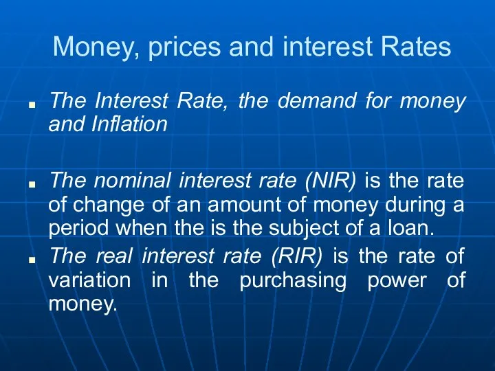
Money, prices and interest Rates
The Interest Rate, the demand for money
Money, prices and interest Rates
The Interest Rate, the demand for money
Money, prices and interest Rates
The Interest Rate, the demand for money
Money, prices and interest Rates
The Interest Rate, the demand for money
Money, prices and interest Rates
The Interest Rate, the demand for money
Money, prices and interest Rates
The Interest Rate, the demand for money
Money, prices and interest Rates
Interest rate and money demand
Md/P =
Money, prices and interest Rates
Interest rate and money demand
Md/P =
Money, prices and interest Rates
The money supply and expected price level
M/P
Money, prices and interest Rates
The money supply and expected price level
M/P
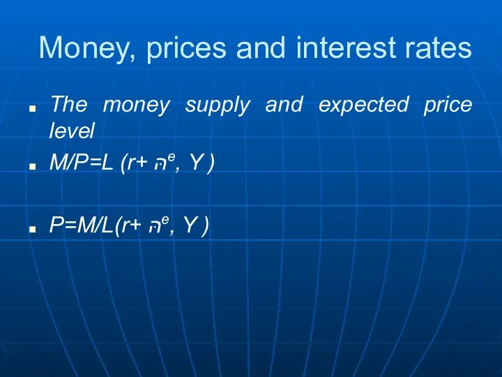
Money, prices and interest rates
The money supply and expected price level
M/P=L
Money, prices and interest rates
The money supply and expected price level
M/P=L
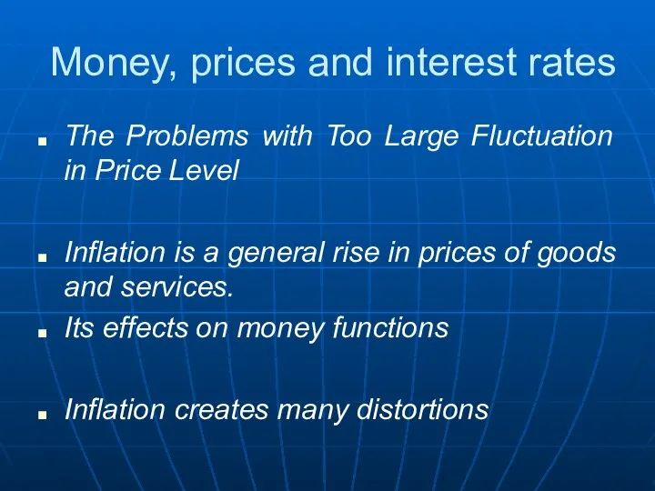
Money, prices and interest rates
The Problems with Too Large Fluctuation in
Money, prices and interest rates
The Problems with Too Large Fluctuation in
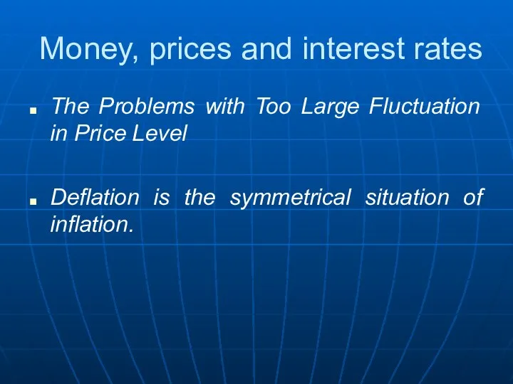
Money, prices and interest rates
The Problems with Too Large Fluctuation in
Money, prices and interest rates
The Problems with Too Large Fluctuation in
Labour market, employment, unemployment
Labour demand comes from com-panies that want to
Labour market, employment, unemployment
Labour demand comes from com-panies that want to
Labour market, employment, unemployment
The labour force is an aggregate that includes
Labour market, employment, unemployment
The labour force is an aggregate that includes
Labour market, employment, unemployment
The labour force is an aggregate that includes
Labour market, employment, unemployment
The labour force is an aggregate that includes
Labour market, employment, unemployment
The labour force is an aggregate that includes
Labour market, employment, unemployment
The labour force is an aggregate that includes
Labour market, employment, unemployment
N=E+U+I N=15-64 years old
a= (E+U)/N
e=E/N
u=U/(E+U)
a=e/(1-u)
Labour market, employment, unemployment
N=E+U+I N=15-64 years old
a= (E+U)/N
e=E/N
u=U/(E+U)
a=e/(1-u)
Labour market, employment, unemployment
Share of long length unemployed (those unemployed for
Labour market, employment, unemployment
Share of long length unemployed (those unemployed for
Labour market, employment, unemployment
The flow of workers
It is the number of
Labour market, employment, unemployment
The flow of workers
It is the number of
The Long-Run Rate of Unemployment
L =E+U
u=U/L
Job acquisition rate a=A/U
The Long-Run Rate of Unemployment
L =E+U
u=U/L
Job acquisition rate a=A/U
The Long-Run Rate of Unemployment
L =E+U
u=U/L
Job loss rate p=P/U
The Long-Run Rate of Unemployment
L =E+U
u=U/L
Job loss rate p=P/U
The Long-Run Rate of Unemployment
Natural rate of unemployment=long-run rate of unemployment
A=P
The Long-Run Rate of Unemployment
Natural rate of unemployment=long-run rate of unemployment
A=P
Economic fluctuations
The economy is experiencing fluctuations that result in variations in
Economic fluctuations
The economy is experiencing fluctuations that result in variations in
Economic fluctuations
Acceleration phases (economic boom)
Contraction phase (economic recession)
Economic fluctuations
Acceleration phases (economic boom)
Contraction phase (economic recession)
Economic fluctuations
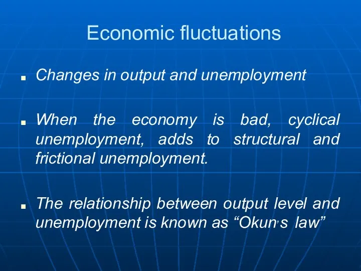
Changes in output and unemployment
When the economy is bad,
Economic fluctuations
Changes in output and unemployment
When the economy is bad,
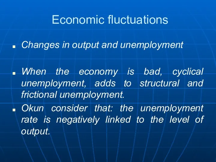
Economic fluctuations
Changes in output and unemployment
When the economy is bad,
Economic fluctuations
Changes in output and unemployment
When the economy is bad,
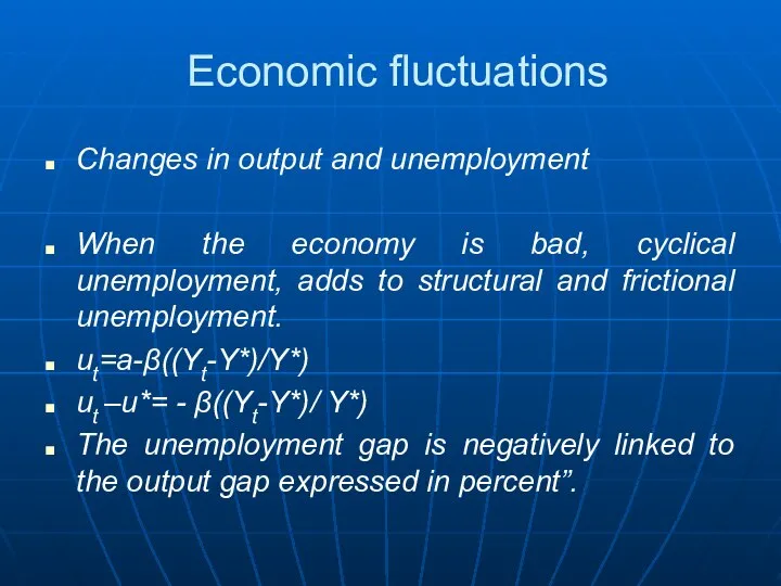
Economic fluctuations
Changes in output and unemployment
When the economy is bad,
Economic fluctuations
Changes in output and unemployment
When the economy is bad,
Economic fluctuations
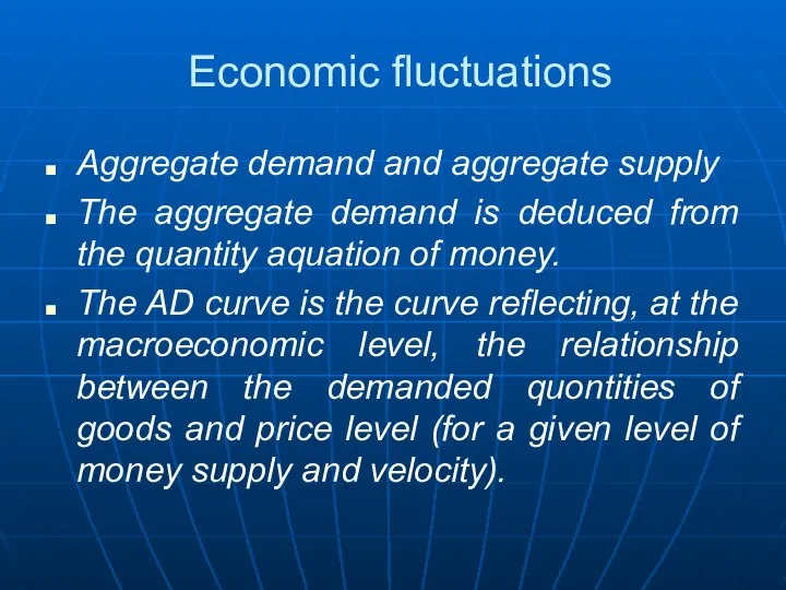
Aggregate demand and aggregate supply
The aggregate demand is deduced
Economic fluctuations
Aggregate demand and aggregate supply
The aggregate demand is deduced
Economic fluctuations
Aggregate demand and aggregate supply
The aggregate supply
The long-run aggregate
Economic fluctuations
Aggregate demand and aggregate supply
The aggregate supply
The long-run aggregate
Economic fluctuations
Aggregate demand and aggregate supply
AS-AD model
Long-run effect of change
Economic fluctuations
Aggregate demand and aggregate supply
AS-AD model
Long-run effect of change
Economic fluctuations
Aggregate demand and aggregate supply
AS-AD model
Short-run effect of change
Economic fluctuations
Aggregate demand and aggregate supply
AS-AD model
Short-run effect of change
Economic fluctuations
Aggregate demand and aggregate supply
AS-AD model
The Effect of Monetary
Economic fluctuations
Aggregate demand and aggregate supply
AS-AD model
The Effect of Monetary
Economic fluctuations
Aggregate demand and aggregate supply
AS-AD model
The Effect of Monetary
Economic fluctuations
Aggregate demand and aggregate supply
AS-AD model
The Effect of Monetary

Economic fluctuations
Aggregate demand and aggregate supply
AS-AD model
The Effect of Monetary
Economic fluctuations
Aggregate demand and aggregate supply
AS-AD model
The Effect of Monetary

Economic fluctuations
Aggregate demand and aggregate supply
AS-AD model
The Effect of Monetary
Economic fluctuations
Aggregate demand and aggregate supply
AS-AD model
The Effect of Monetary
Economic fluctuations
External shock –an event that affects suddenly the economy and
Economic fluctuations
External shock –an event that affects suddenly the economy and
The Keynesian Model of Short-Run Equilibrium
Model IS-LM
Keynesian Macroeconomics (KM)
-
The Keynesian Model of Short-Run Equilibrium
Model IS-LM
Keynesian Macroeconomics (KM)
-
The Keynesian Model of Short-Run Equilibrium
Model IS-LM
Keynesian Macroeconomics (KM)
The Keynesian Model of Short-Run Equilibrium
Model IS-LM
Keynesian Macroeconomics (KM)
The Keynesian Model of Short-Run Equilibrium
Model IS-LM
The impact of budget
The Keynesian Model of Short-Run Equilibrium
Model IS-LM
The impact of budget
The Keynesian Model of Short-Run Equilibrium
Model IS-LM
The impact of budget
The Keynesian Model of Short-Run Equilibrium
Model IS-LM
The impact of budget
The Keynesian Model of Short-Run Equilibrium
Model IS-LM
I =I(r)
IS curve
The Keynesian Model of Short-Run Equilibrium
Model IS-LM
I =I(r)
IS curve
The Keynesian Model of Short-Run Equilibrium
Model IS-LM
Budget policy and IS-curve
The Keynesian Model of Short-Run Equilibrium
Model IS-LM
Budget policy and IS-curve
The Keynesian Model of Short-Run Equilibrium
Model IS-LM
Money market and LM
The Keynesian Model of Short-Run Equilibrium
Model IS-LM
Money market and LM
The Keynesian Model of Short-Run Equilibrium
Model IS-LM
Money market and LM
The Keynesian Model of Short-Run Equilibrium
Model IS-LM
Money market and LM
The Keynesian Model of Short-Run Equilibrium
Model IS-LM
Definition: the LM curve
The Keynesian Model of Short-Run Equilibrium
Model IS-LM
Definition: the LM curve
The Keynesian Model of Short-Run Equilibrium
Model IS-LM
Short-Run Equilibrium
Y=C(Y-T)+I(r)+G
M/P=L(i,Y)
The Keynesian Model of Short-Run Equilibrium
Model IS-LM
Short-Run Equilibrium
Y=C(Y-T)+I(r)+G
M/P=L(i,Y)
The Keynesian Model of Short-Run Equilibrium
Model IS-LM
Economic Policy through the
The Keynesian Model of Short-Run Equilibrium
Model IS-LM
Economic Policy through the
The Keynesian Model of Short-Run Equilibrium
Model IS-LM
Economic Policy through the
The Keynesian Model of Short-Run Equilibrium
Model IS-LM
Economic Policy through the
The Keynesian Model of Short-Run Equilibrium
Model IS-LM
IS-LM and aggregate demand
IS-LM
The Keynesian Model of Short-Run Equilibrium
Model IS-LM
IS-LM and aggregate demand
IS-LM
Aggregate Supply
LRAS –level of output is determined only by amounts of
Aggregate Supply
LRAS –level of output is determined only by amounts of
Aggregate Supply
Nominal wage rigidity
w=W/Pe
W/P=wxPe/P
Aggregate Supply
Nominal wage rigidity
w=W/Pe
W/P=wxPe/P
 Вклад российских ученых в развитие мировой экономической мысли
 Международное кооперативное движение
 Презентация Экономика страны в зеркале международных рейтингов (страна Германия)
 SWOT-анализ
  Offshoring and reshoring
 Экономический анализ контрактов
 Життя Вільяма Петті як основоположника класичної політичної економії в Англії в ХVII - ХVІІІ століттях
 «Statistica» ортасында статистикалық талдау
 Санкт-Петербург. Внешние связи региона
 Государственные и муниципальные преференции
 Петрозаводск - исполнение поручений
 Технопарки России. Технопарк Сколково
 Структура предприятия и организация производственного процесса
 Әлеуметтік – экономикалық дамудағы дағдарыс түсінігі және оның пайда болу себептері
 Презентация Великая Французкая революция 1789-1794 гг
 Предприятия сферы услуг
 Экономика организации
 Международно-правовая база применения нетарифных мер во внешней торговле
 Розвиток національних економік європейських країн в системі світового господарства під впливом науково-технічної революції
 Управление проектом производства молочной продукции на примере К(Ф)Х ИП Воробьев И.А. Хвалынского района Саратовской области
 Економічні потреби
 Зеленая экономика в Казахстане
 Сучасні теорії глобалізації
 Исторический опыт прогнозирования
 Основные макроэкономические показатели. (Часть 3)
 Фирма: издержки производства и прибыль
 Тренды технологического рынка
 Круговорот ресурсов, продукта, дохода. Экономические агенты и их интересы