- Modeling and forecasting. Volatility

Содержание
- 2. Outline Introduction: Why ARCH? ARCH Models Extensions: GARCH, T-GARCH, Q-GARCH, GARCH-M, Box-Cox GARCH Estimation Multivariate GARCH
- 3. 1. Introduction: Why ARCH?
- 4. Why ARCH? ARMA and VAR models are based on the conditional mean of the distribution where
- 5. Some example series: UST10Y
- 6. Dow Jones Symmetric Shocks? Homoskedastic?
- 7. U.S. Unemployment rate vs. stock market volatility, 1929-2010
- 8. U.S. Realized Volatility (kernel based) 1997-2009
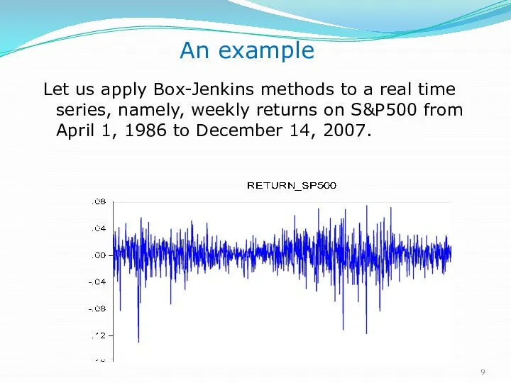
- 9. An example Let us apply Box-Jenkins methods to a real time series, namely, weekly returns on
- 10. Example (cont.) Note: Tranquil period Volatile period
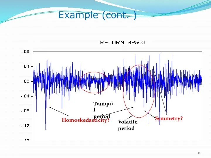
- 11. Example (cont. ) Homoskedasticity? Symmetry? Tranquil period Volatile period
- 12. Example (cont.) Both ACF and PACF are flat, suggesting p=0 and q=0 if we stay in
- 13. Example (cont. ) Look at the histogram and some summary statistics of the data: Asymmetry Fat
- 14. Skewness The shape of a uni-modal distribution can be symmetric or skewed to one side. If
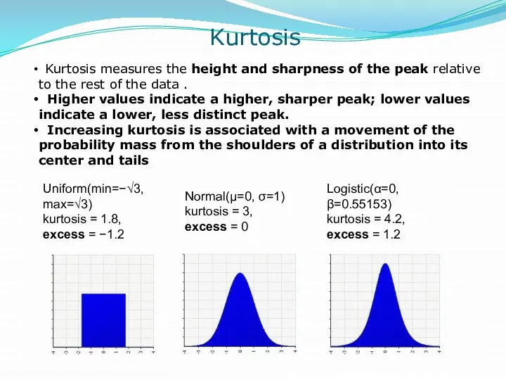
- 15. Kurtosis Kurtosis measures the height and sharpness of the peak relative to the rest of the
- 16. Remarks Gaussian ARMA models are not able to generate asymmetric or fat-tailed behavior. The previous time
- 17. Example Variance of financial returns is often referred to as volatility. To understand the dynamics of
- 18. EViews Example – Daily S&P 500 Returns
- 19. When we learn about GARCH(1,1)…
- 20. We’ll be able to make squared residuals white noise
- 21. Quality of TGARCH predictions: 1% quantiles, VaR(0.01), from August 1, 2007
- 22. 2. ARCH Models
- 24. ARCH(q) AR(J)-ARCH(q) AR(J)-ARCH(q) ARCH(q) Steady-State
- 25. A special case: ARCH(1) Properties [It-1 = y1,..,yt-1] with the AR coefficient γ1 If , the
- 26. Testing for the ARCH effects Regress on . Calculate , which is an LM statistic. Under
- 27. 3. Extensions
- 28. GARCH(p,q) AR(J)-ARCH(q) AR(J)-GARCH(p,q) GARCH(p,q) Steady-State Additivity No negativity
- 29. GARCH(1,1) The most popular ARCH-type model Volatility ( ) VaR=1.645σ
- 30. Properties of GARCH(1,1) 1. follows an ARMA(1,1) with the AR coefficient , and the MA coefficient
- 31. I-GARCH If the coefficients of the GARCH model sum to 1, then the model has “integrated”
- 32. The speed of decrease in the IRFs is determined by Impulse response functions (IRFs) of GARCH(1,1)
- 33. NIC: as a function of holding other variables constant. The NIC of GARCH(1,1): It is symmetric.
- 34. Student t -- GARCH(1,1) where Compared to the Gaussian GARCH, the Student t-GARCH can generate fatter
- 35. T-GARCH (Asymmetry) NIC is asymmetric. If , bad news has a larger impact on the future
- 36. IRFs T-GARCH (Asymmetry)
- 37. NIC is asymmetric as long as Asymmetric Volatility Q(uadratic)-GARCH (Asymmetry)
- 38. NIC of Quadratic GARCH vs. Symmetric GARCH
- 39. GARCH-M An important application of the ARCH-type models is in modeling the trade-off between the mean
- 40. Box-Cox GARCH(1,1) We model the power transformation of volatility. As long as , NIC is asymmetric
- 41. Summary: NICs of Alternative ARCHs Inflation Volatility
- 42. Summing up (see Appendix for an expanded list) Asymmetric Models Non linear
- 43. 3. Estimation
- 44. Maximum Likelihood Maximize L(y,Φ) Φ L*
- 45. Maximum Likelihood (continued) The maximum likelihood decomposes in a “mean” and a “variance” component. Estimation has
- 46. Optimization Newton’s Method Stochastic Newton Method Gradient and Hill Climbing Techniques
- 47. Multiple Solutions Monte Carlo Genetic Algorithms
- 48. 4. Multivariate models
- 49. Multivariate GARCH Models A natural extension of the time-varying variance models based on the univariate GARCH
- 50. Vech Model (2 variables) The conditional variance of each variable depends on its own lagged value,
- 51. BEKK Model C is a NxN lower triangular matrix of unknown parameters A and B are
- 52. Diagonal Vech Model (2 variables) Variances and covariances are GARCH(1,1) Parameters are now 9 instead of
- 53. CCC (Constant Conditional Correlation) Model 3 variables The correlation coefficients are all time invariant
- 54. An extension: VAR + CCC 3 variables
- 55. A further extension: VAR + CCC+ GARCH-M Interactions between Markets Contagion
- 56. An example of volatility “contagion’’
- 57. 5. Application: Value-at-Risk (VaR)
- 58. VaR What is the most I can lose on an investment? VaR tries to provide an
- 59. Value-at-Risk (VaR) VaR summarizes the expected maximum loss over a time horizon within a given confidence
- 60. Value-at-Risk (VaR) - Continued The simplest assumption: daily gains/losses are normally distributed and independent. Calculate VaR
- 61. Measuring VaR with historical data 0 20 40 60 80 100 120 140 160 180 -15
- 62. Assuming a Normal distribution Mean Return (μ) Standard Deviation (σ) Assume that asset returns are normally
- 63. VaR with Normally Distributed Returns The probability of the return falling below a certain threshold depends
- 64. Portfolio VaR When we have more than one asset in our portfolio we can exploit the
- 65. An Example Let us consider the following investment US$200 million invested in 5-year zero coupon US
- 66. An Example (cont.) Suppose we want to compute the 95% VaR. The critical threshold is 1.65
- 67. An Example of Portfolio VaR Two securities 30-year zero-coupon U.S. Treasury bond 5-year zero-coupon U.S. Treasury
- 68. An Example of Portfolio VaR 95% confidence level 30 year zero VaR 1.65 * 0.01409 *
- 69. VaR of the Portfolio Suppose the correlation between the two bonds is ρ12=0.88 Remember that Portfolio
- 70. The problem with Normality: Kurtosis Extreme asset price changes occur more often than the normal distribution
- 71. Fat Tails and underestimation of VaR If we assume that returns are normally distributed when they
- 72. Backtesting Model backtesting involves systematic comparisons of the calculated VaRs with the subsequent realized profits and
- 73. Relevance: Basel VaR Guidelines VaR computed daily, holding period is 10 days. The confidence interval is
- 74. Summing up A host of research has examined a. how best to compute VaR with assumptions
- 75. Thank you!
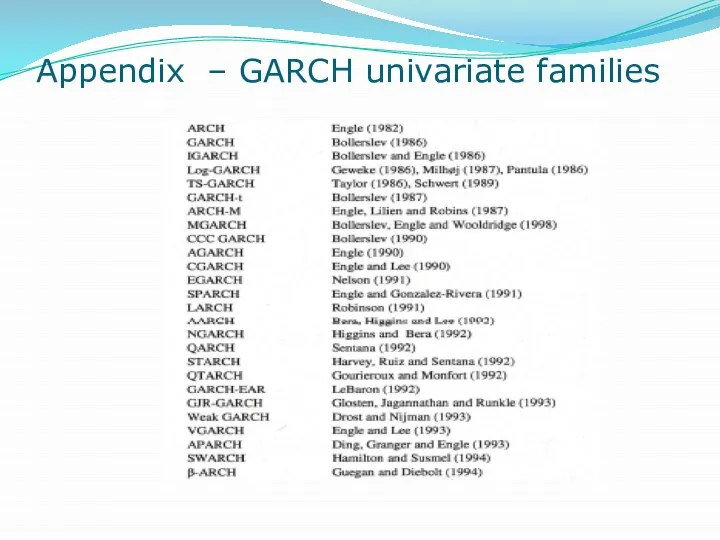
- 76. Appendix – GARCH univariate families
- 77. Source: Bollerslev 2010, Engle Festschrift
- 79. APPENDIX II – Software
- 81. Скачать презентацию

Outline
Introduction: Why ARCH?
ARCH Models
Extensions: GARCH, T-GARCH, Q-GARCH, GARCH-M, Box-Cox GARCH
Estimation
Multivariate GARCH
Outline
Introduction: Why ARCH?
ARCH Models
Extensions: GARCH, T-GARCH, Q-GARCH, GARCH-M, Box-Cox GARCH
Estimation
Multivariate GARCH

1. Introduction:
Why ARCH?
1. Introduction:
Why ARCH?

Why ARCH?
ARMA and VAR models are based on the conditional mean
Why ARCH?
ARMA and VAR models are based on the conditional mean

Some example series: UST10Y
Some example series: UST10Y

Dow Jones
Symmetric Shocks?
Homoskedastic?
Dow Jones
Symmetric Shocks?
Homoskedastic?
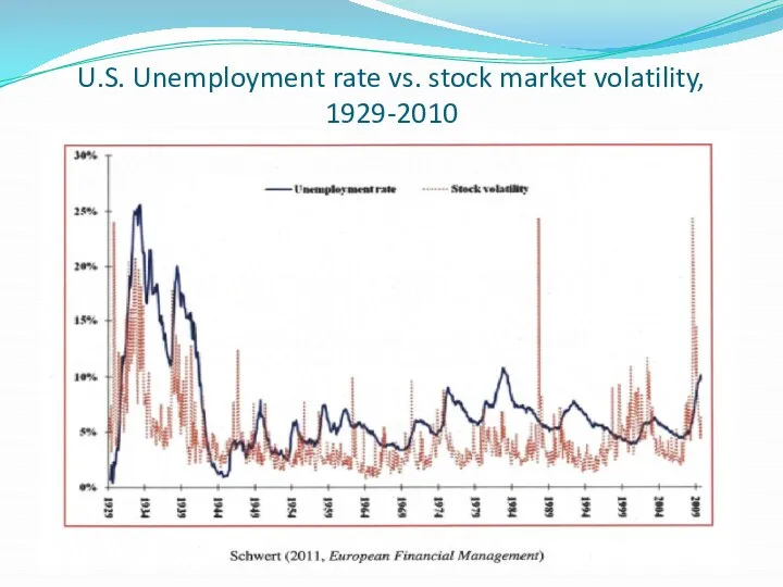
U.S. Unemployment rate vs. stock market volatility, 1929-2010
U.S. Unemployment rate vs. stock market volatility, 1929-2010

U.S. Realized Volatility (kernel based)
1997-2009
U.S. Realized Volatility (kernel based)
1997-2009
An example
Let us apply Box-Jenkins methods to a real time series,
An example
Let us apply Box-Jenkins methods to a real time series,

Example (cont.)
Note:
Tranquil
period
Volatile period
Example (cont.)
Note:
Tranquil
period
Volatile period
Example (cont. )
Homoskedasticity?
Symmetry?
Tranquil
period
Volatile period
Example (cont. )
Homoskedasticity?
Symmetry?
Tranquil
period
Volatile period

Example (cont.)
Both ACF and PACF are flat, suggesting p=0 and q=0
Example (cont.)
Both ACF and PACF are flat, suggesting p=0 and q=0

Example (cont. )
Look at the histogram and some summary statistics of
Example (cont. )
Look at the histogram and some summary statistics of

Skewness
The shape of a uni-modal distribution can be symmetric or
Skewness
The shape of a uni-modal distribution can be symmetric or
Kurtosis
Kurtosis measures the height and sharpness of the peak relative
Kurtosis
Kurtosis measures the height and sharpness of the peak relative

Remarks
Gaussian ARMA models are not able to generate asymmetric or fat-tailed
Remarks
Gaussian ARMA models are not able to generate asymmetric or fat-tailed

Example
Variance of financial returns is often referred to as volatility.
To understand
Example
Variance of financial returns is often referred to as volatility.
To understand

EViews Example – Daily S&P 500 Returns
EViews Example – Daily S&P 500 Returns

When we learn about GARCH(1,1)…
When we learn about GARCH(1,1)…

We’ll be able to make squared residuals white noise
We’ll be able to make squared residuals white noise

Quality of TGARCH predictions: 1% quantiles, VaR(0.01), from August 1, 2007
Quality of TGARCH predictions: 1% quantiles, VaR(0.01), from August 1, 2007
2. ARCH Models
2. ARCH Models

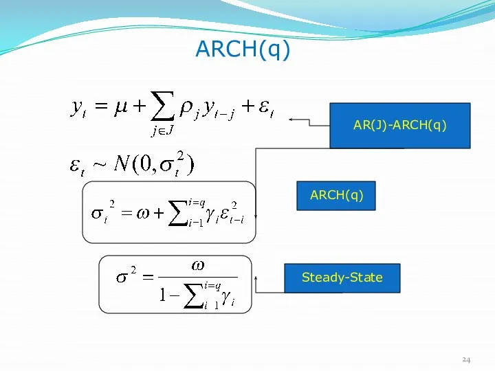
ARCH(q)
AR(J)-ARCH(q)
AR(J)-ARCH(q)
ARCH(q)
Steady-State
ARCH(q)
AR(J)-ARCH(q)
AR(J)-ARCH(q)
ARCH(q)
Steady-State
![A special case: ARCH(1) Properties [It-1 = y1,..,yt-1] with the AR](/_ipx/f_webp&q_80&fit_contain&s_1440x1080/imagesDir/jpg/1434015/slide-24.jpg)
A special case: ARCH(1)
Properties [It-1 = y1,..,yt-1]
with the AR coefficient
A special case: ARCH(1)
Properties [It-1 = y1,..,yt-1]
with the AR coefficient

Testing for the ARCH effects
Regress on .
Calculate , which is
Testing for the ARCH effects
Regress on .
Calculate , which is

3. Extensions
3. Extensions

GARCH(p,q)
AR(J)-ARCH(q)
AR(J)-GARCH(p,q)
GARCH(p,q)
Steady-State
Additivity
No negativity
GARCH(p,q)
AR(J)-ARCH(q)
AR(J)-GARCH(p,q)
GARCH(p,q)
Steady-State
Additivity
No negativity

GARCH(1,1)
The most popular ARCH-type model
Volatility ( )
VaR=1.645σ
GARCH(1,1)
The most popular ARCH-type model
Volatility ( )
VaR=1.645σ

Properties of GARCH(1,1)
1. follows an ARMA(1,1) with the AR coefficient ,
Properties of GARCH(1,1)
1. follows an ARMA(1,1) with the AR coefficient ,

I-GARCH
If the coefficients of the GARCH model sum to 1, then
I-GARCH
If the coefficients of the GARCH model sum to 1, then

The speed of decrease in the IRFs is determined by
Impulse
The speed of decrease in the IRFs is determined by
Impulse
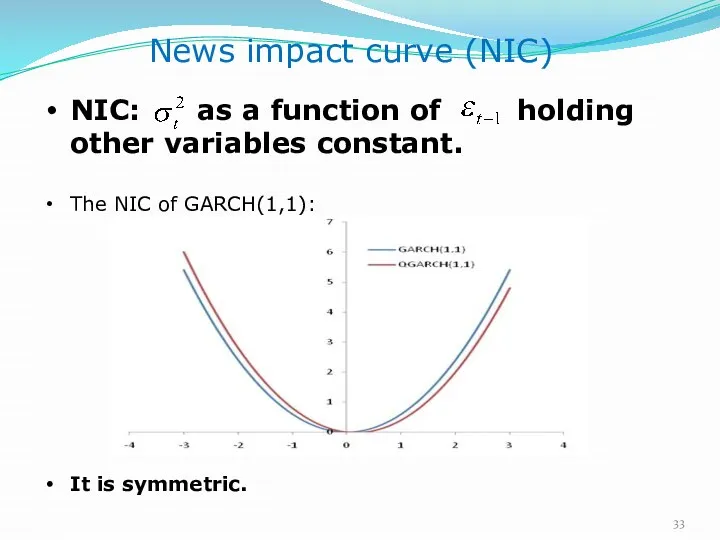
NIC: as a function of holding other variables constant.
The NIC
NIC: as a function of holding other variables constant.
The NIC
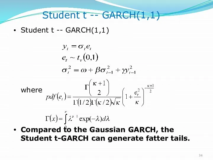
Student t -- GARCH(1,1)
where
Compared to the Gaussian GARCH, the Student t-GARCH
Student t -- GARCH(1,1)
where
Compared to the Gaussian GARCH, the Student t-GARCH
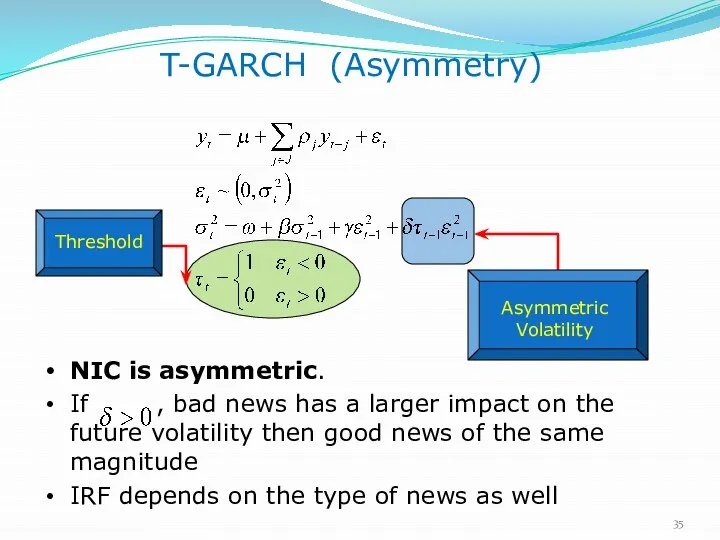
T-GARCH (Asymmetry)
NIC is asymmetric.
If , bad news has a larger
T-GARCH (Asymmetry)
NIC is asymmetric.
If , bad news has a larger

IRFs
T-GARCH (Asymmetry)
IRFs
T-GARCH (Asymmetry)

NIC is asymmetric as long as
Asymmetric Volatility
Q(uadratic)-GARCH (Asymmetry)
NIC is asymmetric as long as
Asymmetric Volatility
Q(uadratic)-GARCH (Asymmetry)
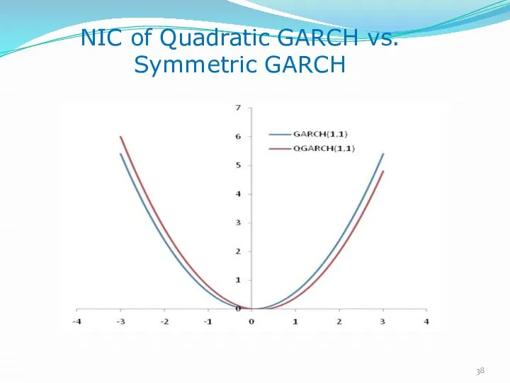
NIC of Quadratic GARCH vs.
Symmetric GARCH
NIC of Quadratic GARCH vs.
Symmetric GARCH

GARCH-M
An important application of the ARCH-type models is in modeling
GARCH-M
An important application of the ARCH-type models is in modeling

Box-Cox GARCH(1,1)
We model the power transformation of volatility.
As long
Box-Cox GARCH(1,1)
We model the power transformation of volatility.
As long
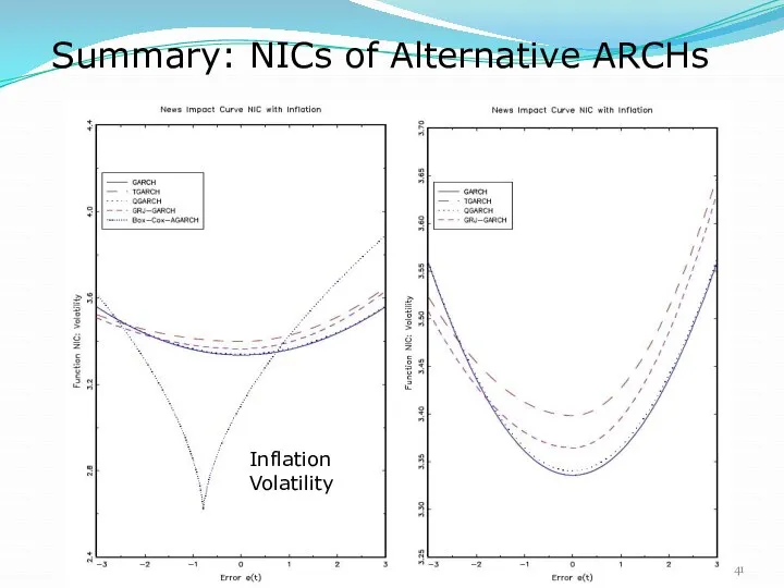
Summary: NICs of Alternative ARCHs
Inflation Volatility
Summary: NICs of Alternative ARCHs
Inflation Volatility

Summing up (see Appendix for an expanded list)
Asymmetric Models
Non linear
Summing up (see Appendix for an expanded list)
Asymmetric Models
Non linear

3. Estimation
3. Estimation
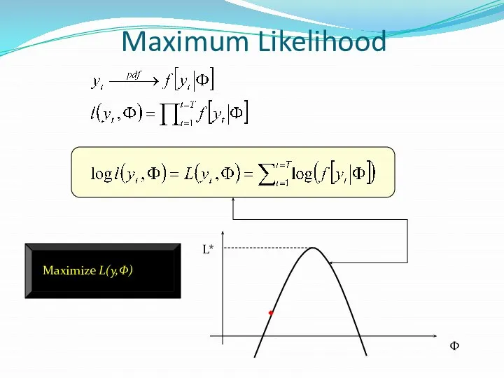
Maximum Likelihood
Maximize L(y,Φ)
Φ
L*
Maximum Likelihood
Maximize L(y,Φ)
Φ
L*

Maximum Likelihood (continued)
The maximum likelihood decomposes in a “mean” and
Maximum Likelihood (continued)
The maximum likelihood decomposes in a “mean” and

Optimization
Newton’s Method
Stochastic Newton Method
Gradient and Hill Climbing Techniques
Optimization
Newton’s Method
Stochastic Newton Method
Gradient and Hill Climbing Techniques

Multiple Solutions
Monte Carlo
Genetic Algorithms
Multiple Solutions
Monte Carlo
Genetic Algorithms

4. Multivariate models
4. Multivariate models

Multivariate GARCH Models
A natural extension of the time-varying variance models based
Multivariate GARCH Models
A natural extension of the time-varying variance models based

Vech Model (2 variables)
The conditional variance of each variable depends on
Vech Model (2 variables)
The conditional variance of each variable depends on

BEKK Model
C is a NxN lower triangular matrix of unknown parameters
BEKK Model
C is a NxN lower triangular matrix of unknown parameters
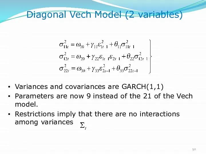
Diagonal Vech Model (2 variables)
Variances and covariances are GARCH(1,1)
Parameters are now
Diagonal Vech Model (2 variables)
Variances and covariances are GARCH(1,1)
Parameters are now

CCC
(Constant Conditional Correlation) Model
3 variables
The correlation coefficients are all time
CCC
(Constant Conditional Correlation) Model
3 variables
The correlation coefficients are all time
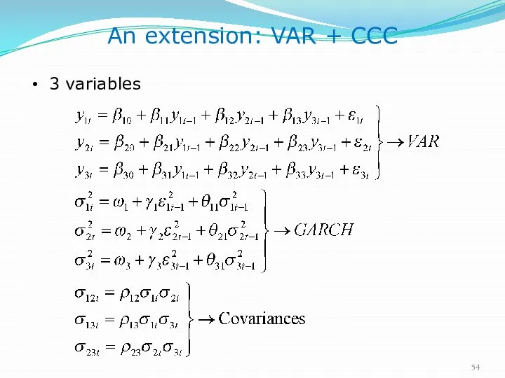
An extension: VAR + CCC
3 variables
An extension: VAR + CCC
3 variables

A further extension:
VAR + CCC+ GARCH-M
Interactions between Markets
Contagion
A further extension:
VAR + CCC+ GARCH-M
Interactions between Markets
Contagion

An example of volatility “contagion’’
An example of volatility “contagion’’

5. Application:
Value-at-Risk (VaR)
5. Application:
Value-at-Risk (VaR)

VaR
What is the most I can lose on an investment?
VaR
VaR
What is the most I can lose on an investment?
VaR

Value-at-Risk (VaR)
VaR summarizes the expected maximum loss over a time horizon
Value-at-Risk (VaR)
VaR summarizes the expected maximum loss over a time horizon

Value-at-Risk (VaR) - Continued
The simplest assumption: daily gains/losses are normally distributed
Value-at-Risk (VaR) - Continued
The simplest assumption: daily gains/losses are normally distributed
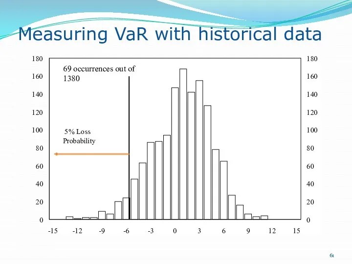
Measuring VaR with historical data
0
20
40
60
80
100
120
140
160
180
-15
-12
-9
-6
-3
0
3
6
9
12
15
0
20
40
60
80
100
120
140
160
180
Probability
Measuring VaR with historical data
0
20
40
60
80
100
120
140
160
180
-15
-12
-9
-6
-3
0
3
6
9
12
15
0
20
40
60
80
100
120
140
160
180
Probability

Assuming a Normal distribution
Mean Return (μ)
Standard Deviation (σ)
Assume that asset returns
Assuming a Normal distribution
Mean Return (μ)
Standard Deviation (σ)
Assume that asset returns

VaR with Normally
Distributed Returns
The probability of the return falling below
VaR with Normally
Distributed Returns
The probability of the return falling below

Portfolio VaR
When we have more than one asset in our portfolio
Portfolio VaR
When we have more than one asset in our portfolio

An Example
Let us consider the following investment
US$200 million invested in 5-year
An Example
Let us consider the following investment
US$200 million invested in 5-year

An Example (cont.)
Suppose we want to compute the 95% VaR.
The
An Example (cont.)
Suppose we want to compute the 95% VaR.
The

An Example of Portfolio VaR
Two securities
30-year zero-coupon U.S. Treasury bond
5-year zero-coupon
An Example of Portfolio VaR
Two securities
30-year zero-coupon U.S. Treasury bond
5-year zero-coupon

An Example of Portfolio VaR
95% confidence level
30 year zero VaR
1.65
An Example of Portfolio VaR
95% confidence level
30 year zero VaR
1.65

VaR of the Portfolio
Suppose the correlation between the two bonds is
VaR of the Portfolio
Suppose the correlation between the two bonds is

The problem with Normality: Kurtosis
Extreme asset price changes occur more often
The problem with Normality: Kurtosis
Extreme asset price changes occur more often

Fat Tails and underestimation of VaR
If we assume that returns are
Fat Tails and underestimation of VaR
If we assume that returns are

Backtesting
Model backtesting involves systematic comparisons of the calculated VaRs with the
Backtesting
Model backtesting involves systematic comparisons of the calculated VaRs with the

Relevance: Basel VaR Guidelines
VaR computed daily, holding period is 10 days.
The
Relevance: Basel VaR Guidelines
VaR computed daily, holding period is 10 days.
The
Summing up
A host of research has examined
a. how best to
Summing up
A host of research has examined
a. how best to

Thank you!
Thank you!
Appendix – GARCH univariate families
Appendix – GARCH univariate families

Source: Bollerslev 2010, Engle Festschrift
Source: Bollerslev 2010, Engle Festschrift


APPENDIX II – Software
APPENDIX II – Software
 Современное состояние и перспективы развития инновационной составляющей экономики Украины
 Предпочтения и выбор
 Борьба с безработицей
 Концептуальные основы регионального развития в России
 Приоритетные направления инновационного развития
 Роль государства в рыночной экономике
 Возникновение экономики и её роль в государстве
 Типы рыночных структур
 Глобализация, её проявления и последствия
 Рынок. Модели. Спрос. Предложение. Равновесие
 Товарная политика. Лекция 3
 Модель кейнсианского креста
 Экономическое взаимодействие России и Китая
 Проект Комфортная городская среда в Великоустюгском муниципальном районе
 Планирование и прогнозирование в условиях рынка
 Методы экономического анализа
 Компанияның қаржы жағдайына жалпы баға беру
 Обмен. Торговля. Реклама (7 класс)
 Рыночные отношения в экономике
 Ключевые этапы реализации стратегии по двигателестроению
 Identification de marché. Identification des clients. Verifier auprés des clients l’attent des produits et services
 Потребности в перемещении людей и товаров,
 Стратегии социального развития России в 21 веке
 Рынок ресурсов
 Презентация Анализ конкурентоспособности экономики
 Поточні витрати торговельного підприємства. (Лекція 12)
 Контрольные цифры проекта бюджета Санкт-Петербурга
 Курсовая работа по методике обучения экономике