- Heat transfer

Содержание
- 2. Introduction to Heat Transfer Heat Conduction Thermal Conductivity Finite Difference Approach for One-Dimensional Steady-State Heat Transfer
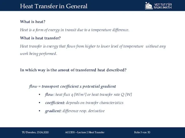
- 3. What is heat? Heat is a form of energy in transit due to a temperature difference.
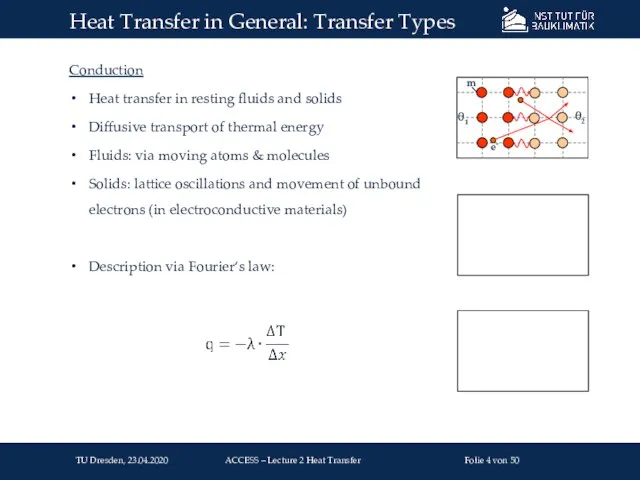
- 4. Conduction Heat transfer in resting fluids and solids Diffusive transport of thermal energy Fluids: via moving
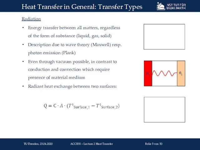
- 5. Radiation Energy transfer between all matters, regardless of the form of substance (liquid, gas, solid) Description
- 6. Convection Heat transfer in/by moving fluid particles 1st transfer via macroscopic resp. bulk motion of the
- 7. Microscopic view: Molecules and atoms are in mutual interaction Particles exchange kinetic energy in chaotic way
- 8. Heat transfer through a solid building construction can be simplified as: Steady- state which assumes time-
- 9. Heat Conduction: 1D TU Dresden, 23.04.2020 Folie von 50 ACCESS – Lecture 2 Heat Transfer T1
- 10. Resulting heat transfer rate (Q) due to heat conduction is: Proportional to the length- related temperature
- 11. Heat Conduction – Thermal Conductivity d R R Influence material thickness: Influence thermal conductivity: Heat transfer
- 12. What is Thermal Conductivity? Thermal conductivity is the ability of a material to conduct heat through
- 13. Heat Conduction: Thermal Conductivity Figure source: M.M.Rathore: Engineering Heat Transfer, Jones & Barlett Learning, 2011 TU
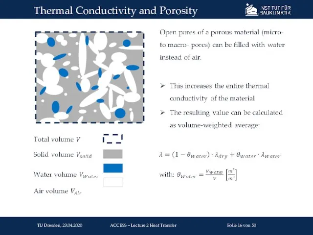
- 14. Thermal Conductivity and Porosity TU Dresden, 23.04.2020 Folie von 50 ACCESS – Lecture 2 Heat Transfer
- 15. Thermal Conductivity and Porosity TU Dresden, 23.04.2020 Folie von 50 ACCESS – Lecture 2 Heat Transfer
- 16. Thermal Conductivity and Porosity TU Dresden, 23.04.2020 Folie von 50 ACCESS – Lecture 2 Heat Transfer
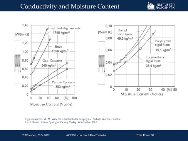
- 17. Conductivity and Moisture Content TU Dresden, 23.04.2020 Folie von 50 ACCESS – Lecture 2 Heat Transfer
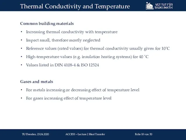
- 18. Common building materials Increasing thermal conductivity with temperature Impact small, therefore mostly neglected Reference values (rated
- 19. Metals: Conductivity is sum of vibration transfer and free electron transfer Free electrons provide huge fraction
- 20. Gases Molecules in continuous random motion Velocity of molecules increases with increasing temperature Thermal Conductivity and
- 21. An isotropic material is a material in which the thermal conductivity does not vary with the
- 22. An insulation material shows an adverse dependency between thermal conductivity and gross density. Example mineral wool:
- 23. Heat Conduction 1D T1 T3 T [K] x [m] T2 T1 x1 x2 dx1-2 dT1-2 dx1-2
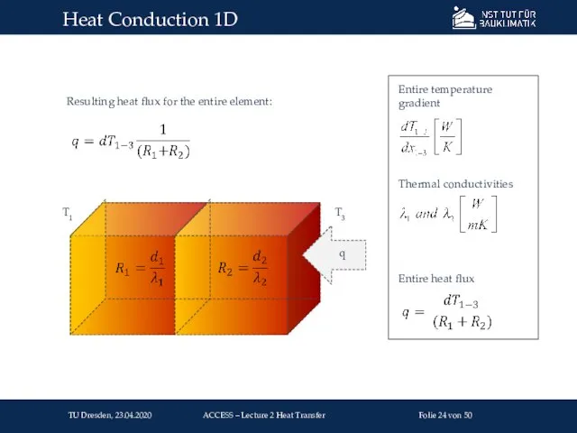
- 24. Heat Conduction 1D T1 T3 Entire temperature gradient Thermal conductivities Entire heat flux q Resulting heat
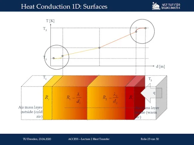
- 25. Heat Conduction 1D: Surfaces T1 T3 Air mass layer outside (cold air) q T1 Air mass
- 26. Surface temperature of a building construction and air mass temperature of the adjacent air mass are
- 27. Heat conduction - Surface Resistance Figure source: www.bradfordinsulation.com.au TU Dresden, 23.04.2020 Folie von 50 ACCESS –
- 28. Heat Conduction - Contact Conditions T [K] T1 T3 Air mass layer outside (cold air) q
- 29. Interface temperature of one material layer and interface temperature of the adjacent material layer are not
- 30. Example: 1D Steady-State Peggy Freudenberg, Building Physics, ACCESS Lime Sand Brick d = 25 cm λ
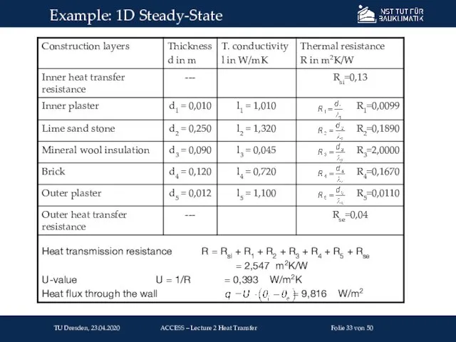
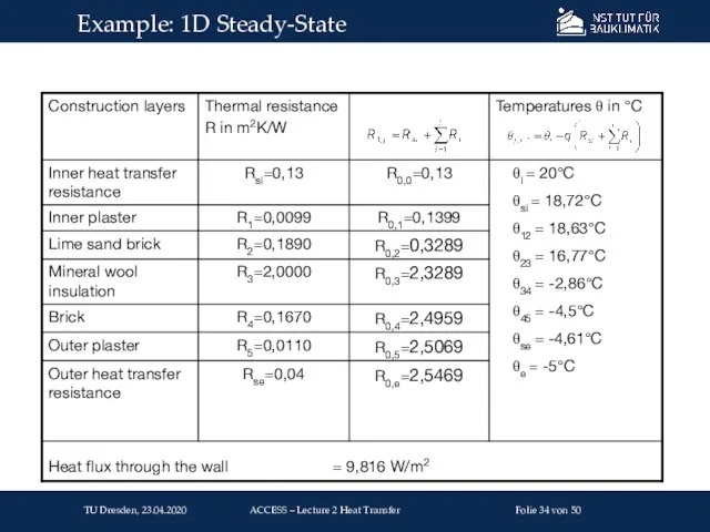
- 31. The heat flux is the same in all layers (steady state): Rearranged as follows: Temperature gradients
- 32. Scheme for the calculation of the steady state temperature profile of a multilayered construction: Calculation heat
- 33. Example: 1D Steady-State TU Dresden, 23.04.2020 Folie von 50 ACCESS – Lecture 2 Heat Transfer
- 34. Example: 1D Steady-State TU Dresden, 23.04.2020 Folie von 50 ACCESS – Lecture 2 Heat Transfer
- 35. In some cases, heat transfer must be seen two-dimensional steady-state: Steady- state assumes Time- constant boundary
- 36. Heat Conduction 2D Steady-State T1 T2 Temperature gradient in x- direction Temperature gradient in y-direction Resulting
- 37. Analytical approaches only for simple geometries and boundary conditions Complex geometries and boundary conditions can be
- 38. Each differential equation is approximated by a finite linear difference equation Construction is divided into equal
- 39. Temperature gradients in x- direction can be transferred into finite difference form Equations for nodes in
- 40. Temperature gradients in y- direction can be transferred into finite difference form in the same way
- 41. Temperature gradient for current (red marked) node is consequently given as: Finite- Difference- Method – 2d
- 42. Applying the 2-dimensional Laplace equation (difference of temperature gradient change in both heat flux directions is
- 43. For the example of control volume method Shape functions describe change of state in each volume
- 44. Example for two- dimensional heat conduction under steady state conditions: Key step is integration of general
- 45. Surface Integral can be evaluated by midpoint rule as: Temperature gradients can be calculated via shape
- 46. Numerical solutions of heat conduction problems offer methods to estimate temperature distribution within an area or
- 47. Dirichlet boundary condition Called boundary condition of first type Temperature at the boundary of the body
- 48. Neumann boundary condition Called boundary condition of second type Heat flux q at the boundary of
- 49. Cauchy boundary condition Called boundary condition of third type Describes correlation between temperature value and derivative
- 50. Advanced Computational and Civil Engineering Structural Studies Exercise 1 Therm (LBNL) Lecturer: P. Freudenberg Contributors: P.
- 51. Therm - overview TU Dresden, 23.04.2020 Folie von 50 ACCESS – Lecture 2 Heat Transfer
- 52. Made up of a finite number of non- overlapping subregions that cover the whole region Well
- 53. Finite element solver: CONRAD Derived from public- domain computer programs TOPAZ2D and FACET Method assumes constant
- 54. Given the wall example you should solve the following tasks: Model this wall example geometry in
- 55. Compute the following tasks for the same external wall example as an edge Model wall example
- 57. Скачать презентацию
Introduction to Heat Transfer
Heat Conduction
Thermal Conductivity
Finite Difference Approach for One-Dimensional Steady-State
Introduction to Heat Transfer
Heat Conduction
Thermal Conductivity
Finite Difference Approach for One-Dimensional Steady-State
What is heat?
Heat is a form of energy in transit due
What is heat?
Heat is a form of energy in transit due
Conduction
Heat transfer in resting fluids and solids
Diffusive transport of thermal energy
Fluids:
Conduction
Heat transfer in resting fluids and solids
Diffusive transport of thermal energy
Fluids:
Radiation
Energy transfer between all matters, regardless of the form of substance
Radiation
Energy transfer between all matters, regardless of the form of substance
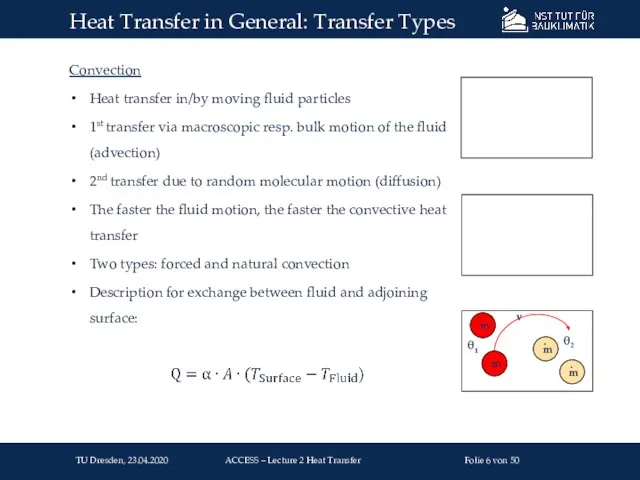
Convection
Heat transfer in/by moving fluid particles
1st transfer via macroscopic resp. bulk
Convection
Heat transfer in/by moving fluid particles
1st transfer via macroscopic resp. bulk
Microscopic view:
Molecules and atoms are in mutual interaction
Particles exchange kinetic energy
Microscopic view:
Molecules and atoms are in mutual interaction
Particles exchange kinetic energy
Heat transfer through a solid building construction can be simplified as:
Steady-
Heat transfer through a solid building construction can be simplified as:
Steady-

Heat Conduction: 1D
TU Dresden, 23.04.2020
Folie von 50
ACCESS – Lecture 2
Heat Conduction: 1D
TU Dresden, 23.04.2020
Folie von 50
ACCESS – Lecture 2

Resulting heat transfer rate (Q) due to heat conduction is:
Proportional to
Resulting heat transfer rate (Q) due to heat conduction is:
Proportional to
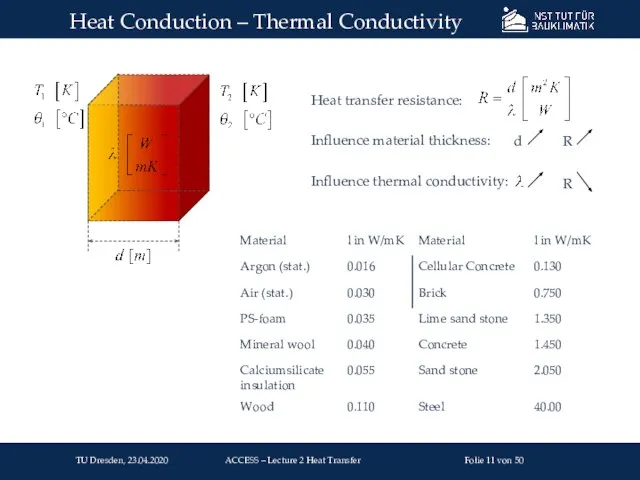
Heat Conduction – Thermal Conductivity
d
R
R
Influence material thickness:
Influence thermal conductivity:
Heat transfer resistance:
TU
Heat Conduction – Thermal Conductivity
d
R
R
Influence material thickness:
Influence thermal conductivity:
Heat transfer resistance:
TU
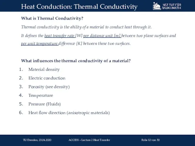
What is Thermal Conductivity?
Thermal conductivity is the ability of a material
What is Thermal Conductivity?
Thermal conductivity is the ability of a material
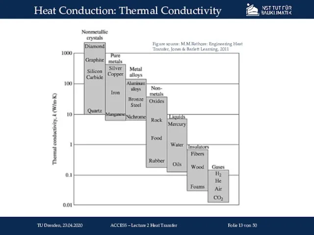
Heat Conduction: Thermal Conductivity
Figure source: M.M.Rathore: Engineering Heat Transfer, Jones &
Heat Conduction: Thermal Conductivity
Figure source: M.M.Rathore: Engineering Heat Transfer, Jones &
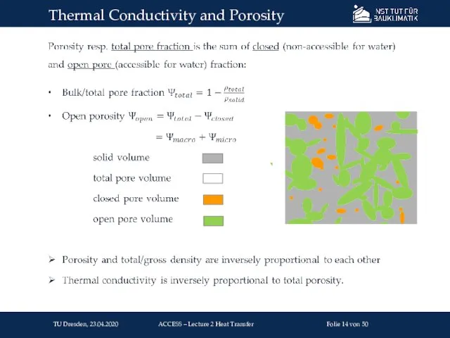
Thermal Conductivity and Porosity
TU Dresden, 23.04.2020
Folie von 50
ACCESS – Lecture 2
Thermal Conductivity and Porosity
TU Dresden, 23.04.2020
Folie von 50
ACCESS – Lecture 2
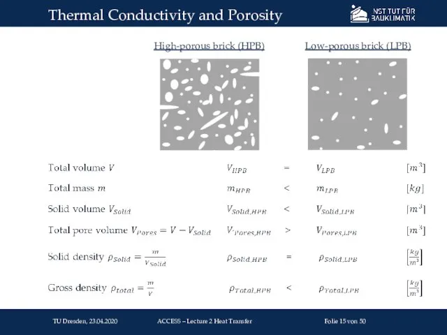
Thermal Conductivity and Porosity
TU Dresden, 23.04.2020
Folie von 50
ACCESS – Lecture 2
Thermal Conductivity and Porosity
TU Dresden, 23.04.2020
Folie von 50
ACCESS – Lecture 2
Thermal Conductivity and Porosity
TU Dresden, 23.04.2020
Folie von 50
ACCESS – Lecture 2
Thermal Conductivity and Porosity
TU Dresden, 23.04.2020
Folie von 50
ACCESS – Lecture 2
Conductivity and Moisture Content
TU Dresden, 23.04.2020
Folie von 50
ACCESS – Lecture 2
Conductivity and Moisture Content
TU Dresden, 23.04.2020
Folie von 50
ACCESS – Lecture 2
Common building materials
Increasing thermal conductivity with temperature
Impact small, therefore mostly
Common building materials
Increasing thermal conductivity with temperature
Impact small, therefore mostly

Metals:
Conductivity is sum of vibration transfer and free electron
Metals:
Conductivity is sum of vibration transfer and free electron
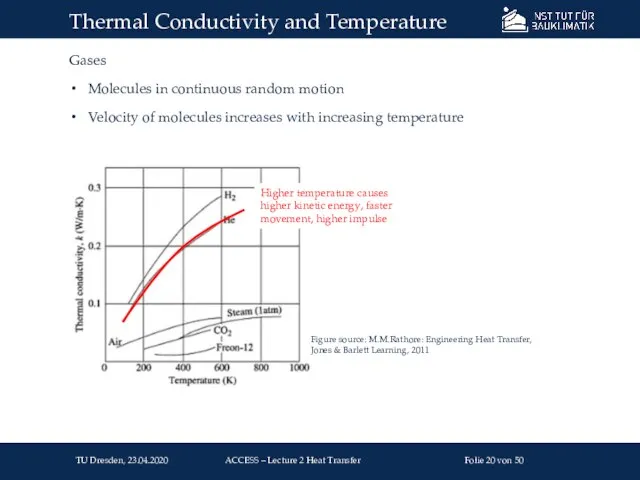
Gases
Molecules in continuous random motion
Velocity of molecules increases with increasing temperature
Thermal
Gases
Molecules in continuous random motion
Velocity of molecules increases with increasing temperature
Thermal
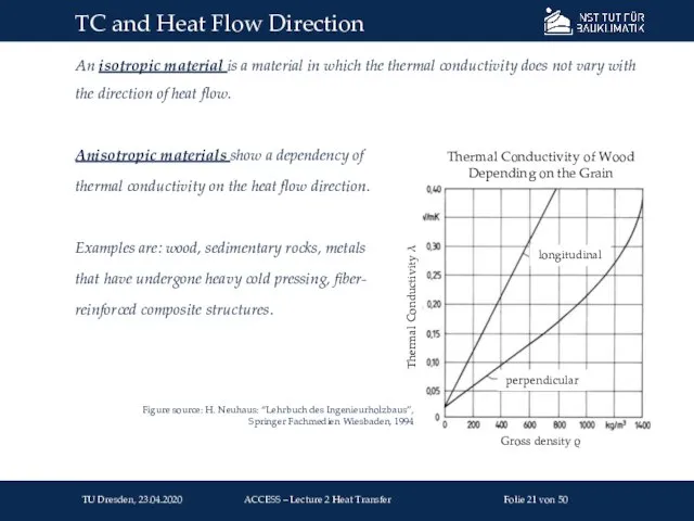
An isotropic material is a material in which the thermal conductivity
An isotropic material is a material in which the thermal conductivity
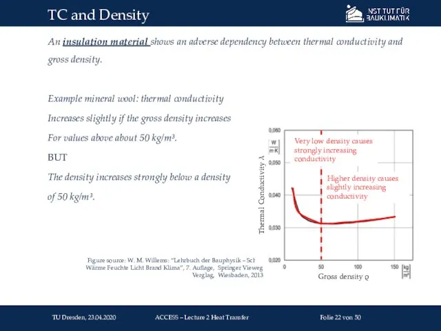
An insulation material shows an adverse dependency between thermal conductivity and
An insulation material shows an adverse dependency between thermal conductivity and
![Heat Conduction 1D T1 T3 T [K] x [m] T2 T1](/_ipx/f_webp&q_80&fit_contain&s_1440x1080/imagesDir/jpg/591446/slide-22.jpg)
Heat Conduction 1D
T1
T3
T [K]
x [m]
T2
T1
x1
x2
dx1-2
dT1-2
dx1-2
Temperature gradients
Thermal conductivities
Resulting heat flux
in
Heat Conduction 1D
T1
T3
T [K]
x [m]
T2
T1
x1
x2
dx1-2
dT1-2
dx1-2
Temperature gradients
Thermal conductivities
Resulting heat flux
in
Heat Conduction 1D
T1
T3
Entire temperature gradient
Thermal conductivities
Entire heat flux
q
Resulting heat flux for
Heat Conduction 1D
T1
T3
Entire temperature gradient
Thermal conductivities
Entire heat flux
q
Resulting heat flux for
Heat Conduction 1D: Surfaces
T1
T3
Air mass layer outside (cold air)
q
T1
Air mass layer
Heat Conduction 1D: Surfaces
T1
T3
Air mass layer outside (cold air)
q
T1
Air mass layer

Surface temperature of a building construction and air mass temperature of
Surface temperature of a building construction and air mass temperature of
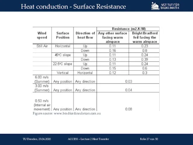
Heat conduction - Surface Resistance
Figure source: www.bradfordinsulation.com.au
TU Dresden, 23.04.2020
Folie von 50
ACCESS
Heat conduction - Surface Resistance
Figure source: www.bradfordinsulation.com.au
TU Dresden, 23.04.2020
Folie von 50
ACCESS
![Heat Conduction - Contact Conditions T [K] T1 T3 Air mass](/_ipx/f_webp&q_80&fit_contain&s_1440x1080/imagesDir/jpg/591446/slide-27.jpg)
Heat Conduction - Contact Conditions
T [K]
T1
T3
Air mass layer outside (cold air)
q
T1
T3
Air
Heat Conduction - Contact Conditions
T [K]
T1
T3
Air mass layer outside (cold air)
q
T1
T3
Air
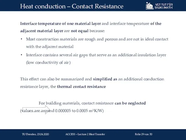
Interface temperature of one material layer and interface temperature of the
Interface temperature of one material layer and interface temperature of the
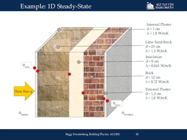
Example: 1D Steady-State
Peggy Freudenberg, Building Physics, ACCESS
Lime Sand Brick
d =
Example: 1D Steady-State
Peggy Freudenberg, Building Physics, ACCESS
Lime Sand Brick
d =
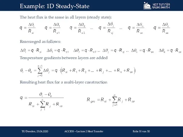
The heat flux is the same in all layers (steady state):
Rearranged
The heat flux is the same in all layers (steady state):
Rearranged
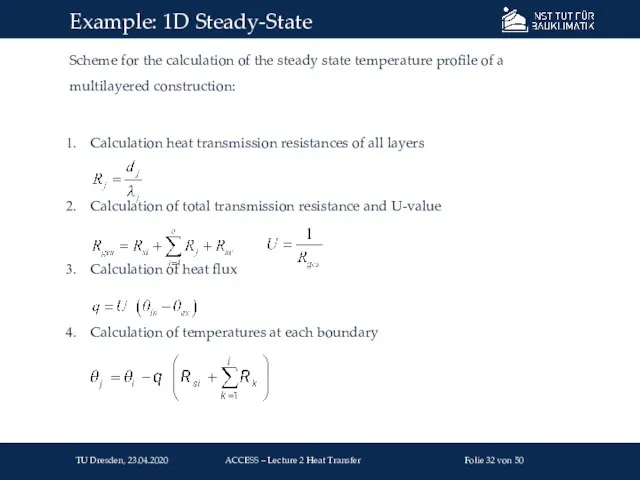
Scheme for the calculation of the steady state temperature profile of
Scheme for the calculation of the steady state temperature profile of
Example: 1D Steady-State
TU Dresden, 23.04.2020
Folie von 50
ACCESS – Lecture 2
Example: 1D Steady-State
TU Dresden, 23.04.2020
Folie von 50
ACCESS – Lecture 2
Example: 1D Steady-State
TU Dresden, 23.04.2020
Folie von 50
ACCESS – Lecture 2
Example: 1D Steady-State
TU Dresden, 23.04.2020
Folie von 50
ACCESS – Lecture 2
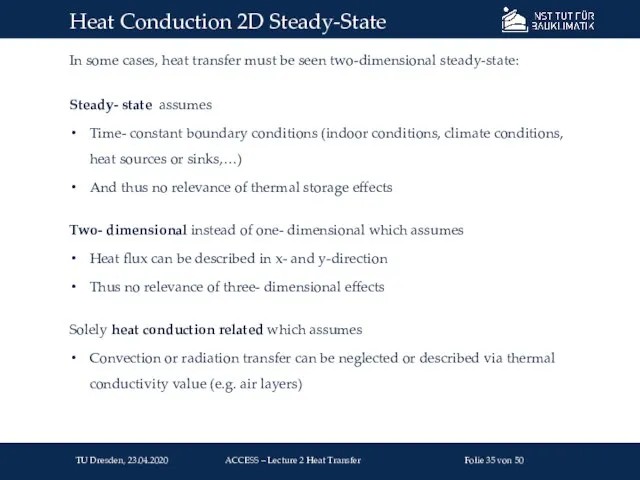
In some cases, heat transfer must be seen two-dimensional steady-state:
Steady- state
In some cases, heat transfer must be seen two-dimensional steady-state:
Steady- state
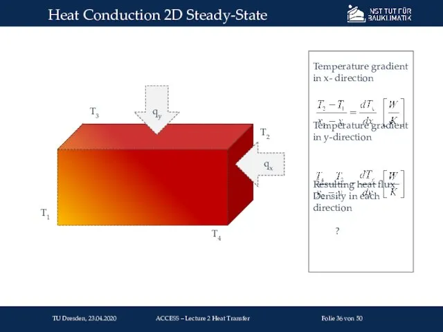
Heat Conduction 2D Steady-State
T1
T2
Temperature gradient in x- direction
Temperature gradient in
Heat Conduction 2D Steady-State
T1
T2
Temperature gradient in x- direction
Temperature gradient in
Analytical approaches only for simple geometries and boundary conditions
Complex geometries and
Analytical approaches only for simple geometries and boundary conditions
Complex geometries and
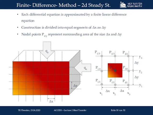
Each differential equation is approximated by a finite linear difference equation
Construction
Each differential equation is approximated by a finite linear difference equation
Construction
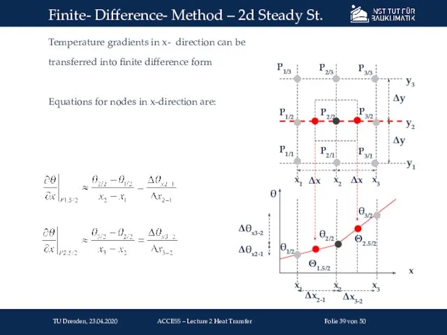
Temperature gradients in x- direction can be
transferred into finite difference
Temperature gradients in x- direction can be
transferred into finite difference
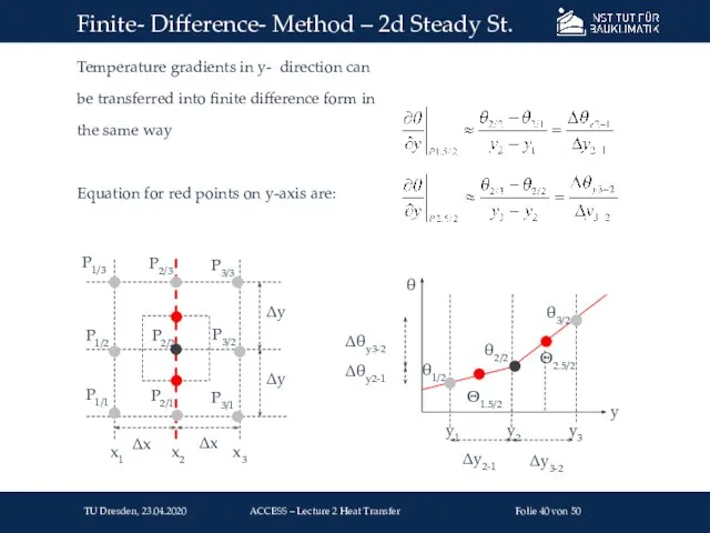
Temperature gradients in y- direction can
be transferred into finite difference
Temperature gradients in y- direction can
be transferred into finite difference
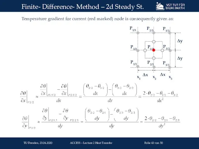
Temperature gradient for current (red marked) node is consequently given as:
Finite-
Temperature gradient for current (red marked) node is consequently given as:
Finite-
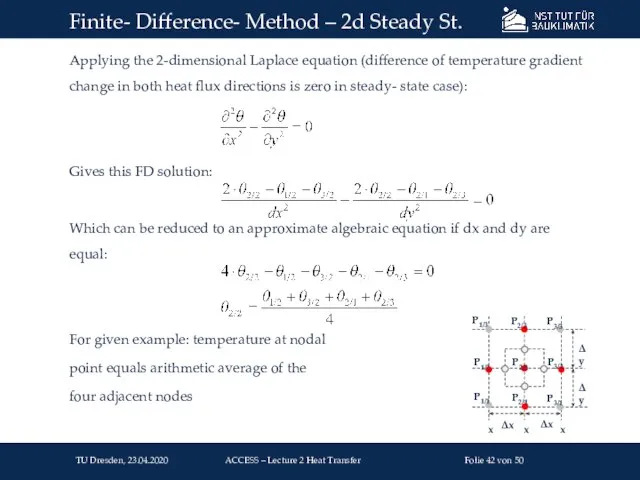
Applying the 2-dimensional Laplace equation (difference of temperature gradient change in
Applying the 2-dimensional Laplace equation (difference of temperature gradient change in
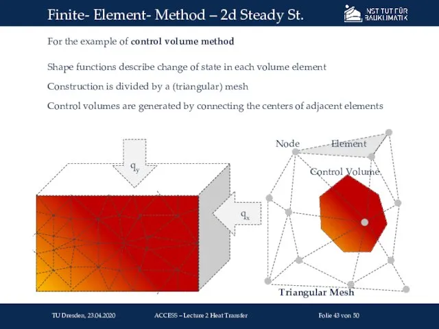
For the example of control volume method
Shape functions describe change of
For the example of control volume method
Shape functions describe change of
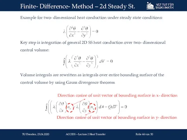
Example for two- dimensional heat conduction under steady state conditions:
Key step
Example for two- dimensional heat conduction under steady state conditions:
Key step
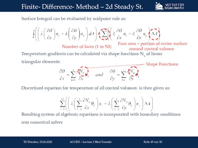
Surface Integral can be evaluated by midpoint rule as:
Temperature gradients can
Surface Integral can be evaluated by midpoint rule as:
Temperature gradients can
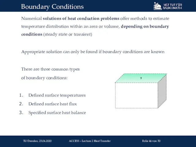
Numerical solutions of heat conduction problems offer methods to estimate temperature
Numerical solutions of heat conduction problems offer methods to estimate temperature
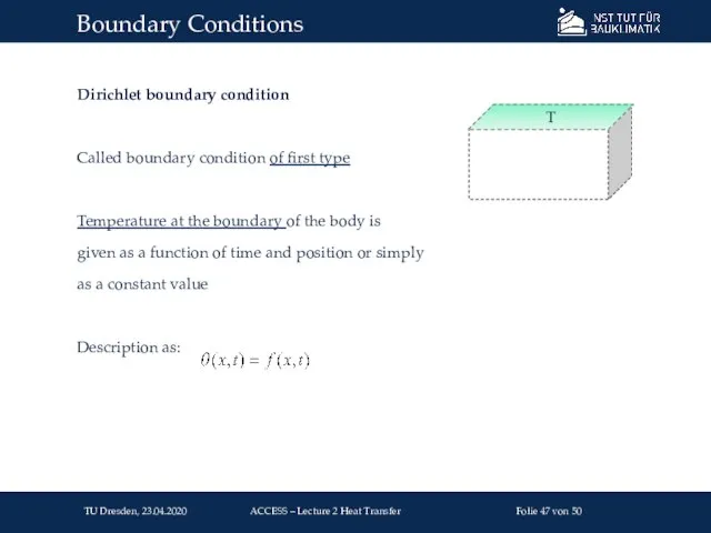
Dirichlet boundary condition
Called boundary condition of first type
Temperature at the boundary
Dirichlet boundary condition
Called boundary condition of first type
Temperature at the boundary
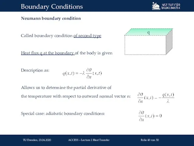
Neumann boundary condition
Called boundary condition of second type
Heat flux q at
Neumann boundary condition
Called boundary condition of second type
Heat flux q at
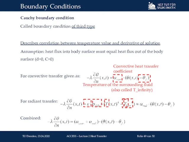
Cauchy boundary condition
Called boundary condition of third type
Describes correlation between temperature
Cauchy boundary condition
Called boundary condition of third type
Describes correlation between temperature
Advanced Computational and Civil Engineering Structural Studies
Exercise 1 Therm (LBNL)
Lecturer:
Advanced Computational and Civil Engineering Structural Studies Exercise 1 Therm (LBNL) Lecturer:
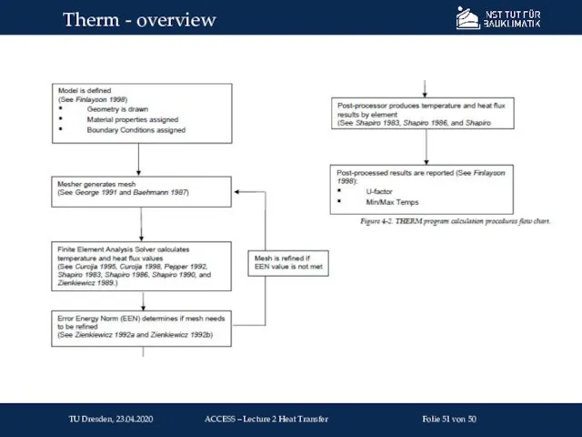
Therm - overview
TU Dresden, 23.04.2020
Folie von 50
ACCESS – Lecture 2 Heat
Therm - overview
TU Dresden, 23.04.2020
Folie von 50
ACCESS – Lecture 2 Heat

Made up of a finite number of non- overlapping subregions that
Made up of a finite number of non- overlapping subregions that

Finite element solver: CONRAD
Derived from public- domain computer programs TOPAZ2D
Finite element solver: CONRAD
Derived from public- domain computer programs TOPAZ2D
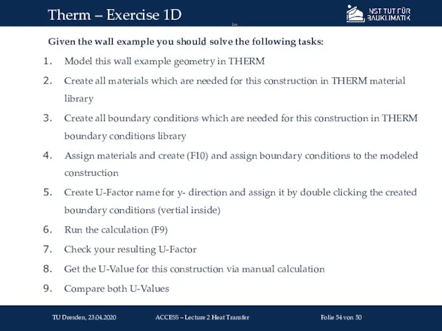
Given the wall example you should solve the following tasks:
Model this
Given the wall example you should solve the following tasks:
Model this
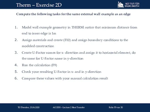
Compute the following tasks for the same external wall example as
Compute the following tasks for the same external wall example as
 Термодинамика биологических процессов
 Учебный курс
  Электромеханический переключатель
 Физические модели. Постановка задачи
 Аккумулятор (лат. accumulator — жинақтауыш) - химиялық реакция энергиясын электр энергиясына айналдыратын аспап; ол электржәне
 Плавание судов
 Сообщающиеся сосуды
 Уравнение Шредингера. Квантовые числа
 Помехи в каналах связи
 Элекромагнитная индукция
 Найзағайдың түрлері
 Механическое движение. Физика 7 класс
 Лазерная технология
 Методы астрофизическиx исследований (МАФИ)
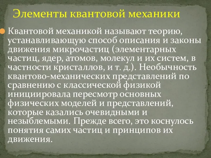 Элементы квантовой механики
 Плоский изгиб. Расчет на прочность
 Физика 8 класс
  Содержание Атомная физика 1.Строение атома (Резерфода) 2.Модель атома водорода по Бору 3.Квантовые постулаты Бора 4.Испускание и п
 Режимы работы электродвигателей по нагреву
 Формирование познавательных интересов у учащихся на уроках физики
 Сила трения
 Решение задач кинетическая и потенциальная энергия
 Резка металла
 Презентация по физике "Транспорт веществ в организме человека. Диффузия. Осмос" - скачать
  Вклад Ломоносова в изучение физики и астрономии.
 Механический электрогенератор
 Эксперимент – как метод обучения естественным наукам
 Понятие динамической системы станка. Динамическое качество станка. Основные задачи динамики станков