- Graphs and Multigraphs

Содержание
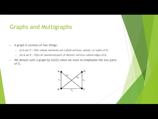
- 2. Graphs and Multigraphs A graph G consists of two things: (i) A set V = V(G)
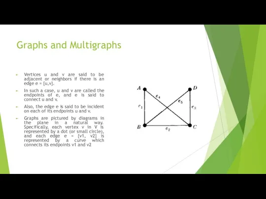
- 3. Graphs and Multigraphs Vertices u and v are said to be adjacent or neighbors if there
- 4. Multigraphs Consider the diagram on the left. The edges e4 and e5 are called multiple edges
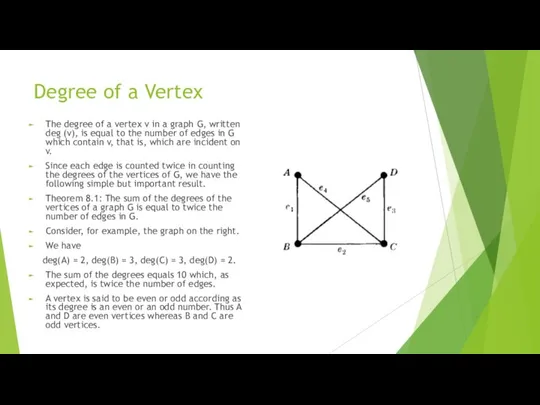
- 5. Degree of a Vertex The degree of a vertex v in a graph G, written deg
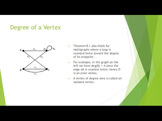
- 6. Degree of a Vertex Theorem 8.1 also holds for multigraphs where a loop is counted twice
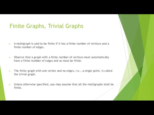
- 7. Finite Graphs, Trivial Graphs A multigraph is said to be finite if it has a finite
- 8. SUBGRAPHS, ISOMORPHICAND HOMEOMORPHIC GRAPHS Subgraphs Consider a graph G = G(V,E).Agraph H = H(V’,E’) is called
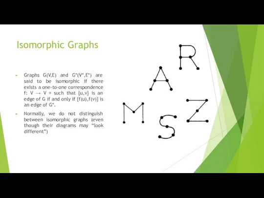
- 9. Isomorphic Graphs Graphs G(V,E) and G*(V*,E*) are said to be isomorphic if there exists a one-to-one
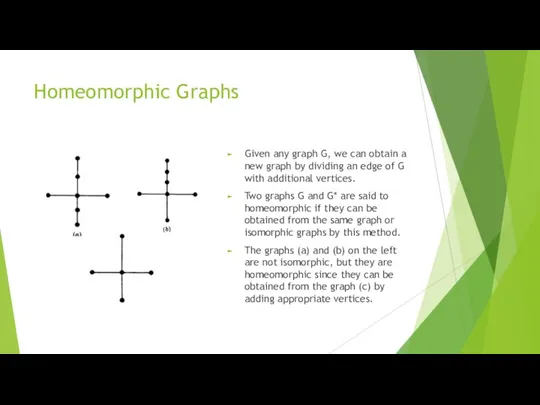
- 10. Homeomorphic Graphs Given any graph G, we can obtain a new graph by dividing an edge
- 11. PATHS
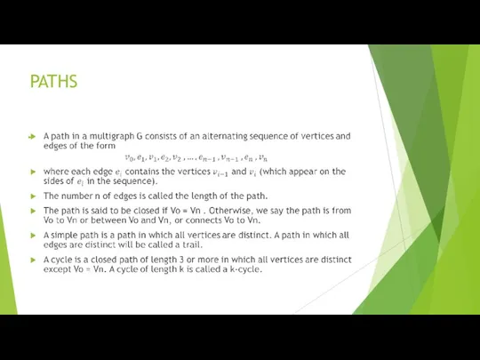
- 12. Paths Consider the following sequences: α = (P4,P1,P2,P5,P1,P2,P3, P6) β = (P4,P1,P5,P2,P6) γ = (P4,P1,P5,P2,P3,P5,P6) The
- 13. Connectivity/Connected Components A graph G is connected if there is a path between any two of
- 14. Distance and Diameter Consider a connected graph G. The distance between vertices u and v in
- 15. Cutpoints and Bridges Let G be a connected graph. A vertex v in G is called
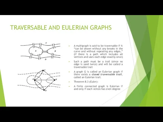
- 16. TRAVERSABLE AND EULERIAN GRAPHS A multigraph is said to be traversable if it “can be drawn
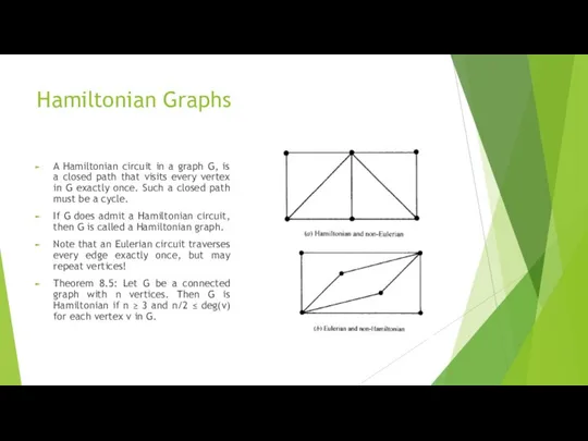
- 17. Hamiltonian Graphs A Hamiltonian circuit in a graph G, is a closed path that visits every
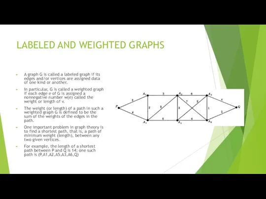
- 18. LABELED AND WEIGHTED GRAPHS A graph G is called a labeled graph if its edges and/or
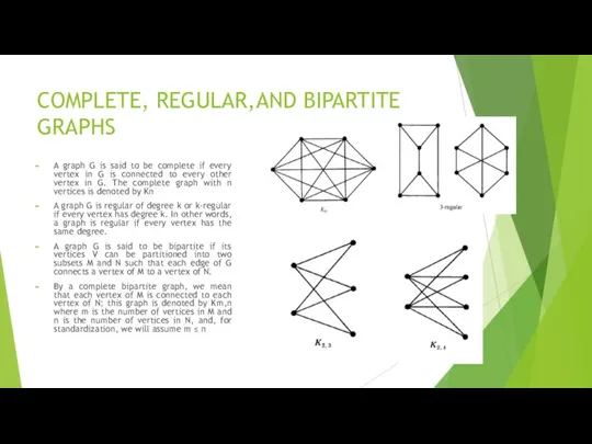
- 19. COMPLETE, REGULAR,AND BIPARTITE GRAPHS A graph G is said to be complete if every vertex in
- 20. Trees A graph T is called a tree if T is connected and T has no
- 21. Trees Theorem 8.6: Let G be a graph with n > 1 vertices. Then the following
- 22. Spanning Trees A subgraph T of a connected graph G is called a spanning tree of
- 23. Minimal Spanning Trees Suppose G is a connected weighted graph. That is, each edge of G
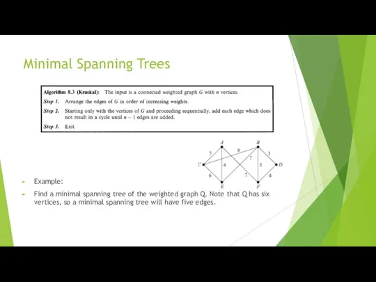
- 24. Minimal Spanning Trees Example: Find a minimal spanning tree of the weighted graph Q. Note that
- 25. First we order the edges by decreasing weights, and then we successively delete edges without disconnecting
- 26. Minimal Spanning Trees Example: Find a minimal spanning tree of the weighted graph Q. Note that
- 27. First we order the edges by increasing weights, and then we successively add edges without forming
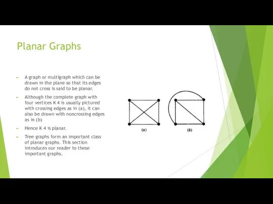
- 28. Planar Graphs A graph or multigraph which can be drawn in the plane so that its
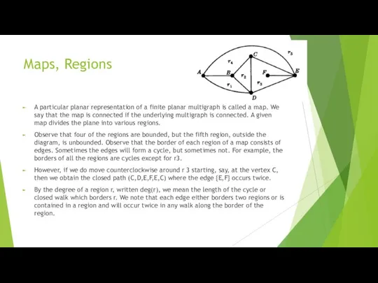
- 29. Maps, Regions A particular planar representation of a finite planar multigraph is called a map. We
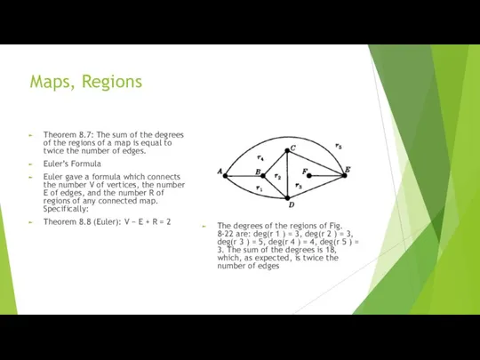
- 30. Maps, Regions Theorem 8.7: The sum of the degrees of the regions of a map is
- 31. Non-planar Graps
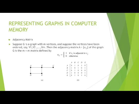
- 32. REPRESENTING GRAPHS IN COMPUTER MEMORY
- 33. REPRESENTING GRAPHS IN COMPUTER MEMORY
- 34. REPRESENTING GRAPHS IN COMPUTER MEMORY The linked representation of a graph G, which maintains G in
- 35. REPRESENTING GRAPHS IN COMPUTER MEMORY Edge File: The Edge File contains the edges of the graph
- 36. REPRESENTING GRAPHS IN COMPUTER MEMORY
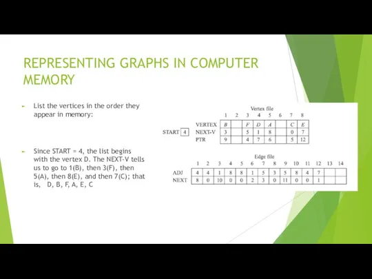
- 37. REPRESENTING GRAPHS IN COMPUTER MEMORY List the vertices in the order they appear in memory: Since
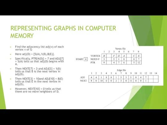
- 38. REPRESENTING GRAPHS IN COMPUTER MEMORY Find the adjacency list adj(v) of each vertex v of G
- 39. GRAPH ALGORITHMS This section discusses two important graph algorithms which systematically examine the vertices and edges
- 40. GRAPH ALGORITHMS During the execution of our algorithms, each vertex (node) N of G will be
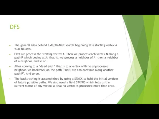
- 41. DFS The general idea behind a depth-first search beginning at a starting vertex A is as
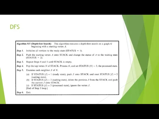
- 42. DFS
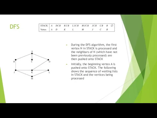
- 43. DFS During the DFS algorithm, the first vertex N in STACK is processed and the neighbors
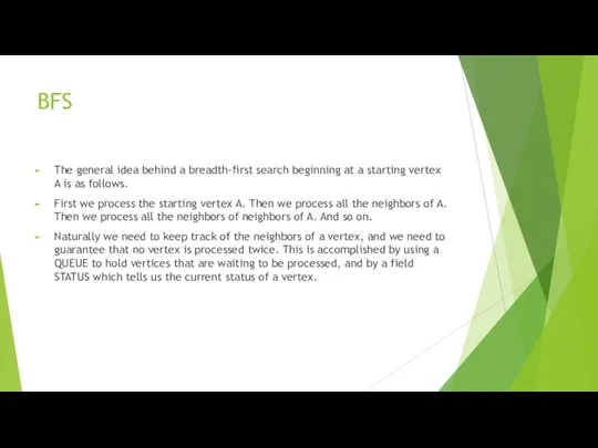
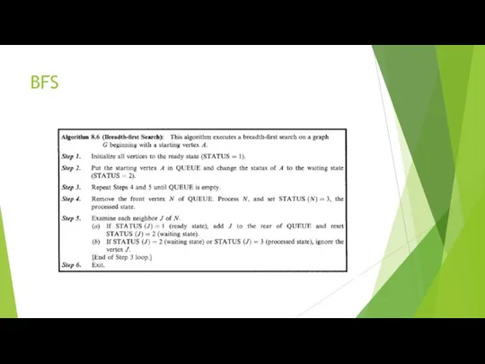
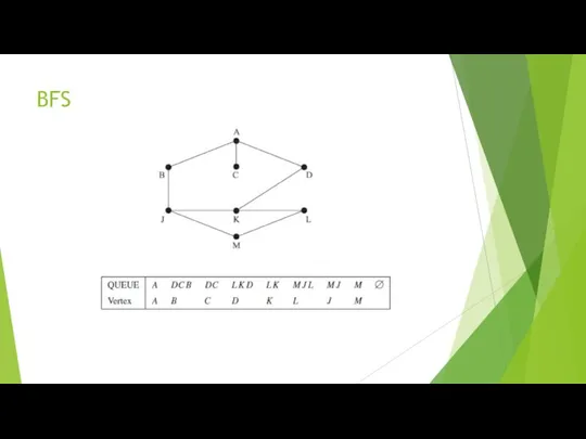
- 44. BFS The general idea behind a breadth-first search beginning at a starting vertex A is as
- 45. BFS
- 46. BFS
- 47. Traveling Salesman Problem Let G be a complete weighted graph. (We view the vertices of G
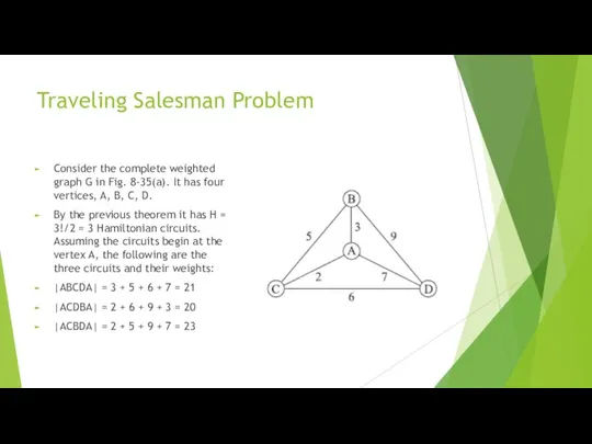
- 48. Traveling Salesman Problem Consider the complete weighted graph G in Fig. 8-35(a). It has four vertices,
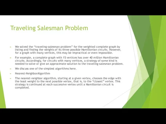
- 49. Traveling Salesman Problem We solved the “traveling-salesman problem” for the weighted complete graph by listing and
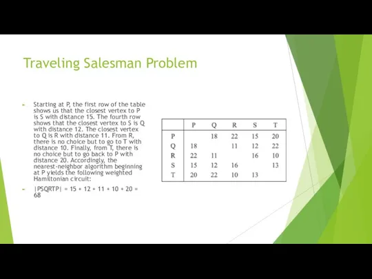
- 50. Traveling Salesman Problem Starting at P, the first row of the table shows us that the
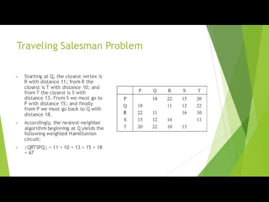
- 51. Traveling Salesman Problem Starting at Q, the closest vertex is R with distance 11; from R
- 53. Скачать презентацию
Graphs and Multigraphs
A graph G consists of two things:
(i) A set
Graphs and Multigraphs
A graph G consists of two things:
(i) A set
Graphs and Multigraphs
Vertices u and v are said to be adjacent
Graphs and Multigraphs
Vertices u and v are said to be adjacent

Multigraphs
Consider the diagram on the left.
The edges e4 and e5 are
Multigraphs
Consider the diagram on the left.
The edges e4 and e5 are
Degree of a Vertex
The degree of a vertex v in a
Degree of a Vertex
The degree of a vertex v in a
Degree of a Vertex
Theorem 8.1 also holds for multigraphs where a
Degree of a Vertex
Theorem 8.1 also holds for multigraphs where a
Finite Graphs, Trivial Graphs
A multigraph is said to be finite if
Finite Graphs, Trivial Graphs
A multigraph is said to be finite if

SUBGRAPHS, ISOMORPHICAND HOMEOMORPHIC GRAPHS
Subgraphs
Consider a graph G = G(V,E).Agraph H =
SUBGRAPHS, ISOMORPHICAND HOMEOMORPHIC GRAPHS
Subgraphs
Consider a graph G = G(V,E).Agraph H =
Isomorphic Graphs
Graphs G(V,E) and G*(V*,E*) are said to be isomorphic if
Isomorphic Graphs
Graphs G(V,E) and G*(V*,E*) are said to be isomorphic if
Homeomorphic Graphs
Given any graph G, we can obtain a new graph
Homeomorphic Graphs
Given any graph G, we can obtain a new graph
PATHS
PATHS
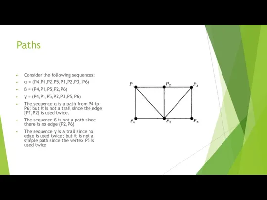
Paths
Consider the following sequences:
α = (P4,P1,P2,P5,P1,P2,P3, P6)
β = (P4,P1,P5,P2,P6)
γ =
Paths
Consider the following sequences:
α = (P4,P1,P2,P5,P1,P2,P3, P6)
β = (P4,P1,P5,P2,P6)
γ =
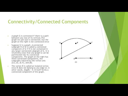
Connectivity/Connected Components
A graph G is connected if there is a path
Connectivity/Connected Components
A graph G is connected if there is a path
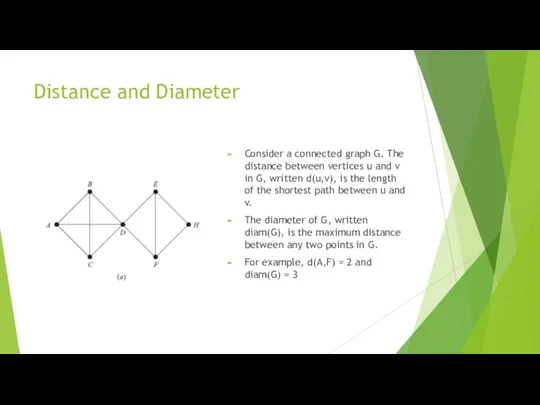
Distance and Diameter
Consider a connected graph G. The distance between vertices
Distance and Diameter
Consider a connected graph G. The distance between vertices
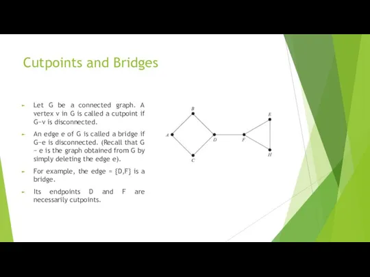
Cutpoints and Bridges
Let G be a connected graph. A vertex v
Cutpoints and Bridges
Let G be a connected graph. A vertex v
TRAVERSABLE AND EULERIAN GRAPHS
A multigraph is said to be traversable if
TRAVERSABLE AND EULERIAN GRAPHS
A multigraph is said to be traversable if
Hamiltonian Graphs
A Hamiltonian circuit in a graph G, is a closed
Hamiltonian Graphs
A Hamiltonian circuit in a graph G, is a closed
LABELED AND WEIGHTED GRAPHS
A graph G is called a labeled graph
LABELED AND WEIGHTED GRAPHS
A graph G is called a labeled graph
COMPLETE, REGULAR,AND BIPARTITE GRAPHS
A graph G is said to be complete
COMPLETE, REGULAR,AND BIPARTITE GRAPHS
A graph G is said to be complete
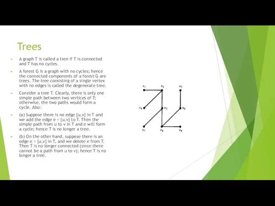
Trees
A graph T is called a tree if T is connected
Trees
A graph T is called a tree if T is connected
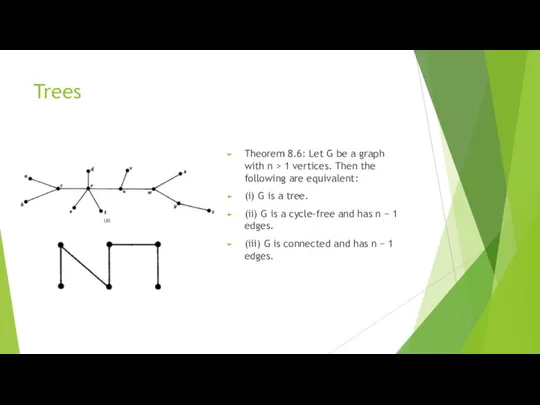
Trees
Theorem 8.6: Let G be a graph with n > 1
Trees
Theorem 8.6: Let G be a graph with n > 1
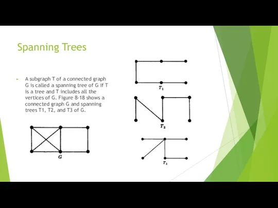
Spanning Trees
A subgraph T of a connected graph G is called
Spanning Trees
A subgraph T of a connected graph G is called

Minimal Spanning Trees
Suppose G is a connected weighted graph. That is,
Minimal Spanning Trees
Suppose G is a connected weighted graph. That is,
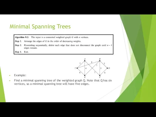
Minimal Spanning Trees
Example:
Find a minimal spanning tree of the weighted
Minimal Spanning Trees
Example:
Find a minimal spanning tree of the weighted
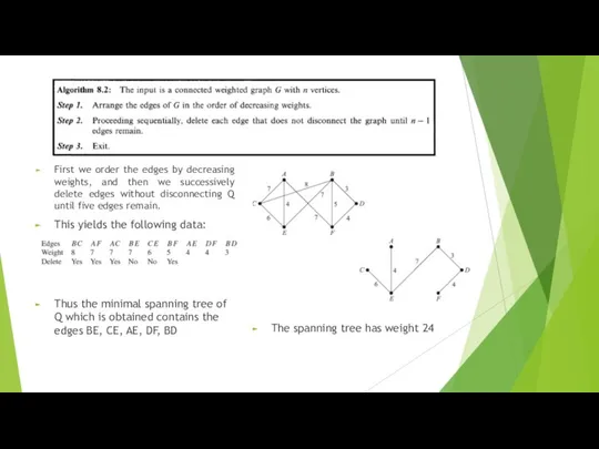
First we order the edges by decreasing weights, and then we
First we order the edges by decreasing weights, and then we
Minimal Spanning Trees
Example:
Find a minimal spanning tree of the weighted
Minimal Spanning Trees
Example:
Find a minimal spanning tree of the weighted
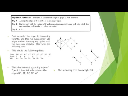
First we order the edges by increasing weights, and then we
First we order the edges by increasing weights, and then we
Planar Graphs
A graph or multigraph which can be drawn in the
Planar Graphs
A graph or multigraph which can be drawn in the
Maps, Regions
A particular planar representation of a finite planar multigraph is
Maps, Regions
A particular planar representation of a finite planar multigraph is
Maps, Regions
Theorem 8.7: The sum of the degrees of the regions
Maps, Regions
Theorem 8.7: The sum of the degrees of the regions
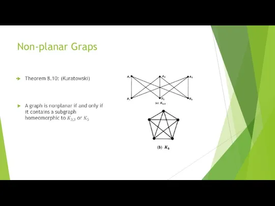
Non-planar Graps
Non-planar Graps
REPRESENTING GRAPHS IN COMPUTER MEMORY
REPRESENTING GRAPHS IN COMPUTER MEMORY
REPRESENTING GRAPHS IN COMPUTER MEMORY
REPRESENTING GRAPHS IN COMPUTER MEMORY
REPRESENTING GRAPHS IN COMPUTER MEMORY
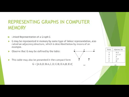
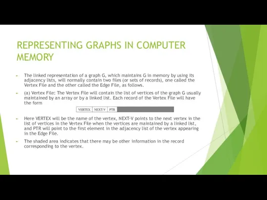
The linked representation of a graph G,
REPRESENTING GRAPHS IN COMPUTER MEMORY
The linked representation of a graph G,
REPRESENTING GRAPHS IN COMPUTER MEMORY
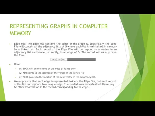
Edge File: The Edge File contains the
REPRESENTING GRAPHS IN COMPUTER MEMORY
Edge File: The Edge File contains the
REPRESENTING GRAPHS IN COMPUTER MEMORY
REPRESENTING GRAPHS IN COMPUTER MEMORY
REPRESENTING GRAPHS IN COMPUTER MEMORY
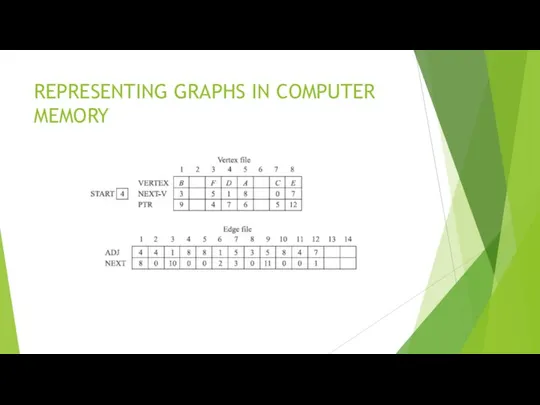
List the vertices in the order they
REPRESENTING GRAPHS IN COMPUTER MEMORY
List the vertices in the order they
REPRESENTING GRAPHS IN COMPUTER MEMORY
Find the adjacency list adj(v) of each
REPRESENTING GRAPHS IN COMPUTER MEMORY
Find the adjacency list adj(v) of each
GRAPH ALGORITHMS
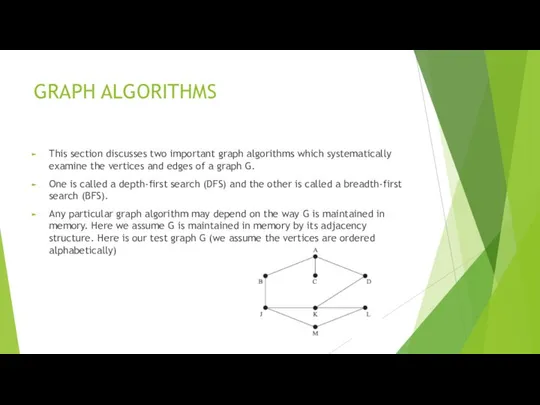
This section discusses two important graph algorithms which systematically examine
GRAPH ALGORITHMS
This section discusses two important graph algorithms which systematically examine
GRAPH ALGORITHMS
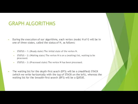
During the execution of our algorithms, each vertex (node) N
GRAPH ALGORITHMS
During the execution of our algorithms, each vertex (node) N
DFS
The general idea behind a depth-first search beginning at a starting
DFS
The general idea behind a depth-first search beginning at a starting
DFS
DFS
DFS
During the DFS algorithm, the first vertex N in STACK is
DFS
During the DFS algorithm, the first vertex N in STACK is
BFS
The general idea behind a breadth-first search beginning at a starting
BFS
The general idea behind a breadth-first search beginning at a starting
BFS
BFS
BFS
BFS
Traveling Salesman Problem
Let G be a complete weighted graph. (We view
Traveling Salesman Problem
Let G be a complete weighted graph. (We view
Traveling Salesman Problem
Consider the complete weighted graph G in Fig. 8-35(a).
Traveling Salesman Problem
Consider the complete weighted graph G in Fig. 8-35(a).
Traveling Salesman Problem
We solved the “traveling-salesman problem” for the weighted complete
Traveling Salesman Problem
We solved the “traveling-salesman problem” for the weighted complete
Traveling Salesman Problem
Starting at P, the first row of the table
Traveling Salesman Problem
Starting at P, the first row of the table
Traveling Salesman Problem
Starting at Q, the closest vertex is R with
Traveling Salesman Problem
Starting at Q, the closest vertex is R with
 Систематическая погрешность
 Презентация на тему ЛУЧ И УГОЛ
  Історія розвитку комбінаторики та деякі її застосування
 Скалярное произведение векторов
 Математика 2 класс Урок разработан учителем начальных классов МОУ «СОШ №48» Крыцыной Еленой Анатольевной
 Формулы приведения
 Предмет стереометрии. Аксиомы стереометрии
 Тема урока. Сложение и вычитание дробей с одинаковыми знаменателями.
 Длина окружности и площадь круга. 6 класс
 Задание 2. Задача минимизировать время сбора утром на работу и в школу семьи из трех человек: отец, сын (10 лет), дочь (6 лет)
 Как показать ученикам, что не всякая формула задает функцию и не всякую функцию можно задать формулой?
 Порядок выполнения действий
 Умножение и деление чисел. Повторение
 Симметрия в пространстве
 Симметрия. Центральная и осевая симметрии
 Отношение двух чисел
 Презентация по математике "Рациональные уравнения" - скачать бесплатно
 Предварительный эксперимент и методы его анализа
 Задачи на движение. Математические модели
 Площадь параллелограмма
 Решение задач на прямую и обратную пропорциональные зависимости
 Измерение физических величин и единицы их измерения
 Тела Архимеда
 Множество. Подмножество
 Доли и части от числа
 Тригонометрические уравнения Практикум по решению и составлению тригонометрических уравнений
 Алғашқы функция және интеграл
 Занимательная математика