- Financial econometrics

Содержание
- 2. Financial Econometrics 2016 – Dr. Kashif Saleem (UOWD) Univariate time series models Univariate time series modelling
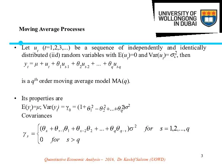
- 3. Quantitative Economic Analysis – 2016, Dr. Kashif Saleem (UOWD) Let ut (t=1,2,3,...) be a sequence of
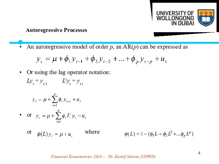
- 4. Financial Econometrics 2016 – Dr. Kashif Saleem (UOWD) An autoregressive model of order p, an AR(p)
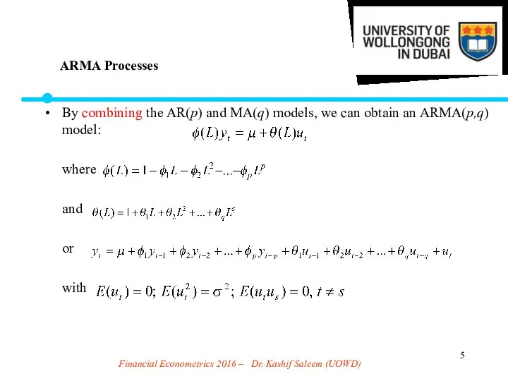
- 5. Financial Econometrics 2016 – Dr. Kashif Saleem (UOWD) By combining the AR(p) and MA(q) models, we
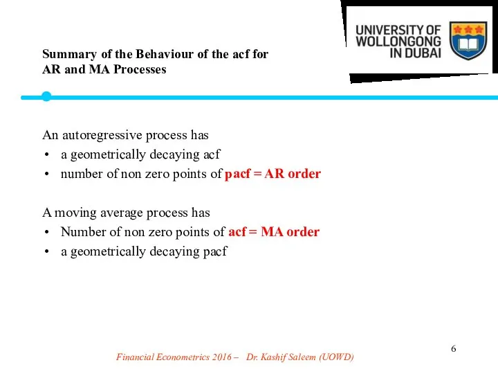
- 6. Financial Econometrics 2016 – Dr. Kashif Saleem (UOWD) An autoregressive process has a geometrically decaying acf
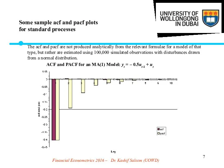
- 7. Financial Econometrics 2016 – Dr. Kashif Saleem (UOWD) The acf and pacf are not produced analytically
- 8. Financial Econometrics 2016 – Dr. Kashif Saleem (UOWD) ACF and PACF for an MA(2) Model: yt
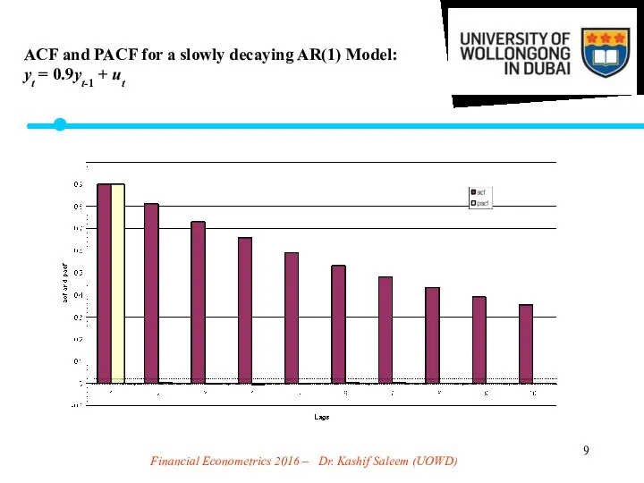
- 9. Financial Econometrics 2016 – Dr. Kashif Saleem (UOWD) ACF and PACF for a slowly decaying AR(1)
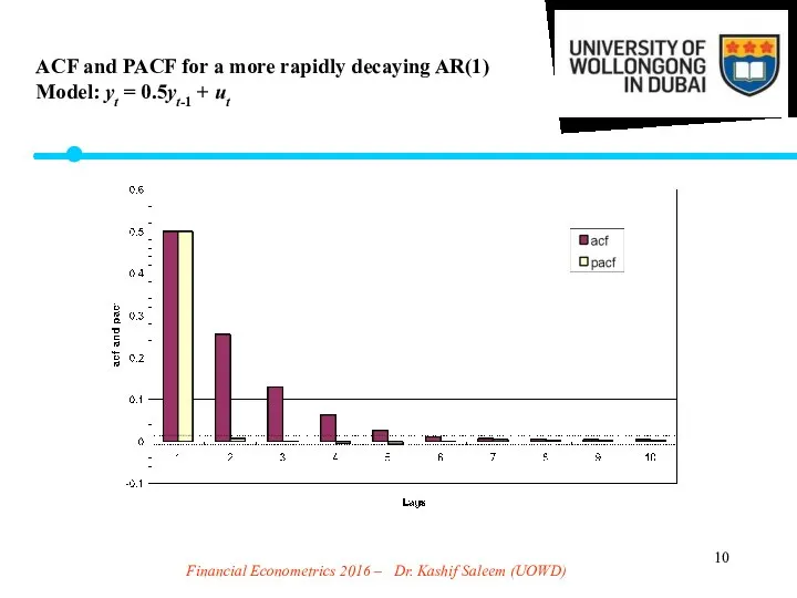
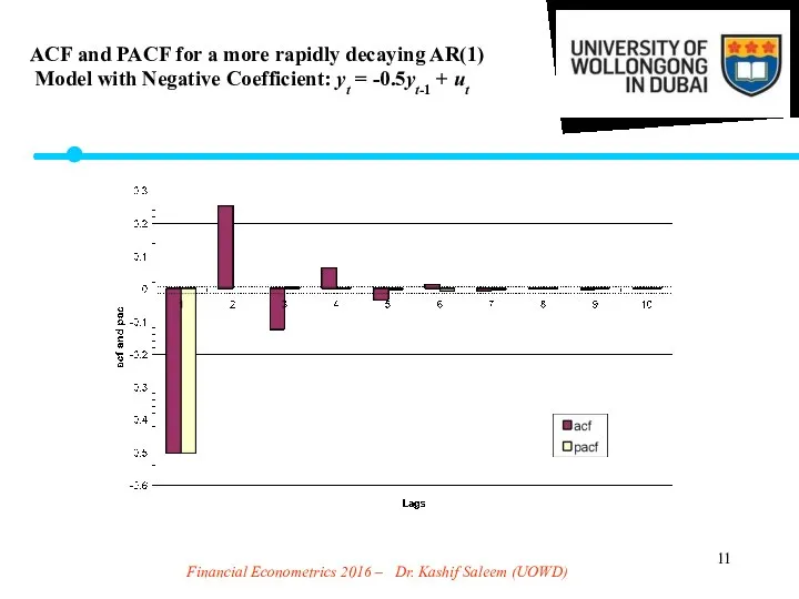
- 10. Financial Econometrics 2016 – Dr. Kashif Saleem (UOWD) ACF and PACF for a more rapidly decaying
- 11. Financial Econometrics 2016 – Dr. Kashif Saleem (UOWD) ACF and PACF for a more rapidly decaying
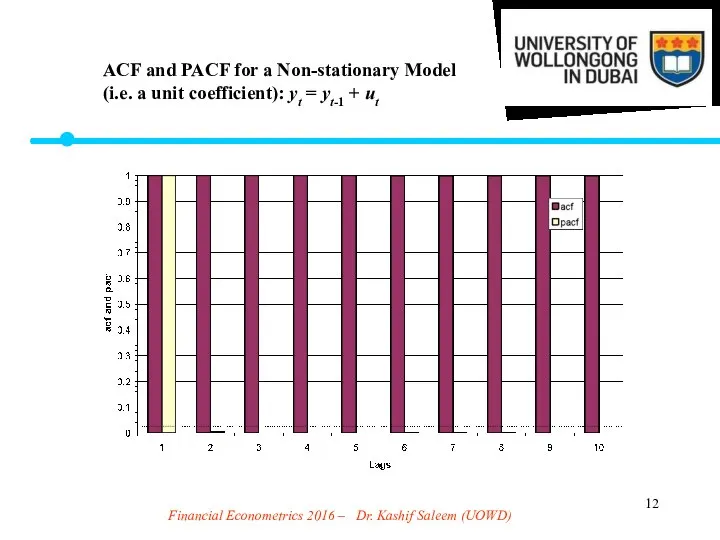
- 12. Financial Econometrics 2016 – Dr. Kashif Saleem (UOWD) ACF and PACF for a Non-stationary Model (i.e.
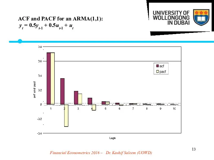
- 13. Financial Econometrics 2016 – Dr. Kashif Saleem (UOWD) ACF and PACF for an ARMA(1,1): yt =
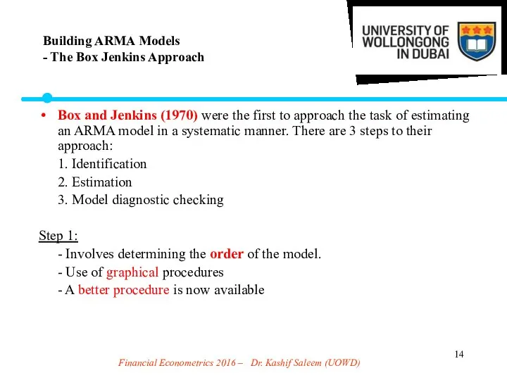
- 14. Financial Econometrics 2016 – Dr. Kashif Saleem (UOWD) Box and Jenkins (1970) were the first to
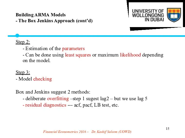
- 15. Financial Econometrics 2016 – Dr. Kashif Saleem (UOWD) Step 2: - Estimation of the parameters -
- 16. Financial Econometrics 2016 – Dr. Kashif Saleem (UOWD) Identification would typically not be done using acf’s.
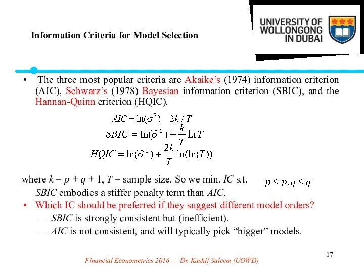
- 17. Financial Econometrics 2016 – Dr. Kashif Saleem (UOWD) The three most popular criteria are Akaike’s (1974)
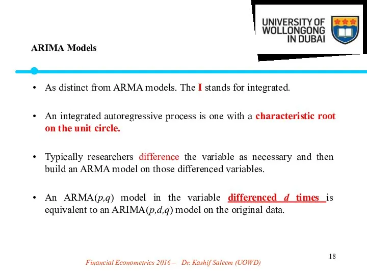
- 18. Financial Econometrics 2016 – Dr. Kashif Saleem (UOWD) As distinct from ARMA models. The I stands
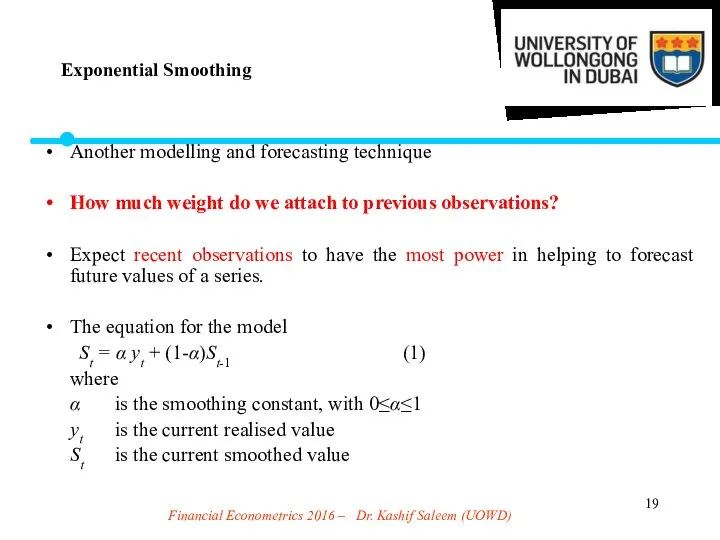
- 19. Financial Econometrics 2016 – Dr. Kashif Saleem (UOWD) Another modelling and forecasting technique How much weight
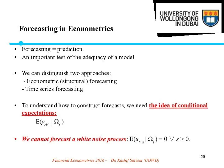
- 20. Financial Econometrics 2016 – Dr. Kashif Saleem (UOWD) Forecasting = prediction. An important test of the
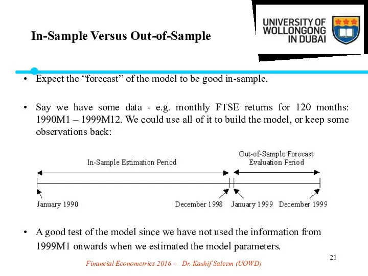
- 21. Financial Econometrics 2016 – Dr. Kashif Saleem (UOWD) Expect the “forecast” of the model to be
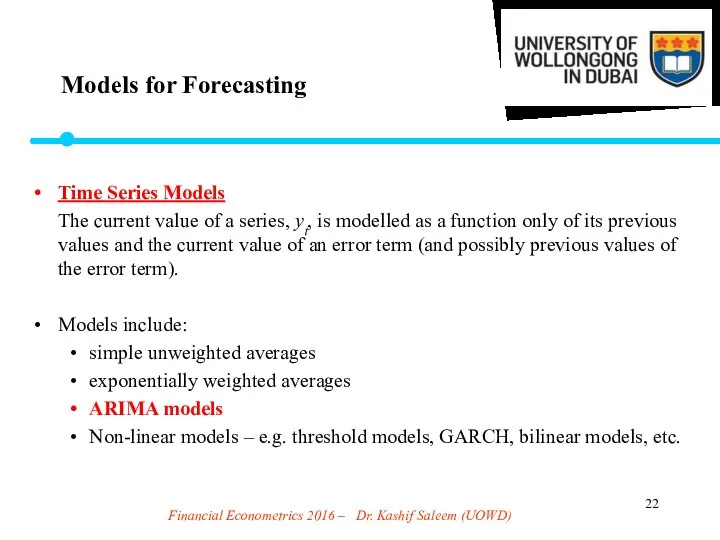
- 22. Financial Econometrics 2016 – Dr. Kashif Saleem (UOWD) Models for Forecasting Time Series Models The current
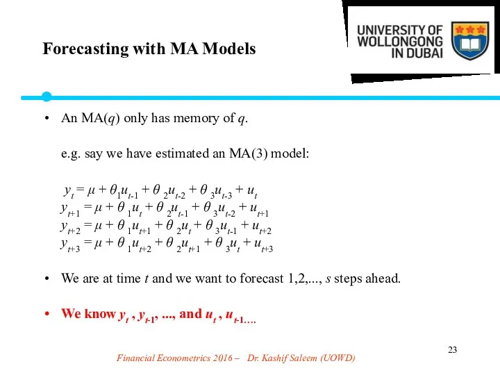
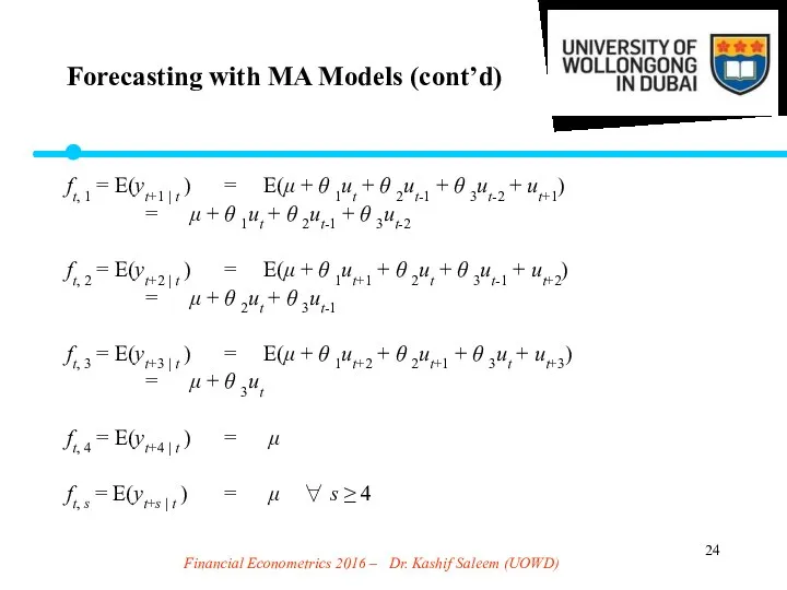
- 23. Financial Econometrics 2016 – Dr. Kashif Saleem (UOWD) An MA(q) only has memory of q. e.g.
- 24. Financial Econometrics 2016 – Dr. Kashif Saleem (UOWD) ft, 1 = E(yt+1 | t ) =
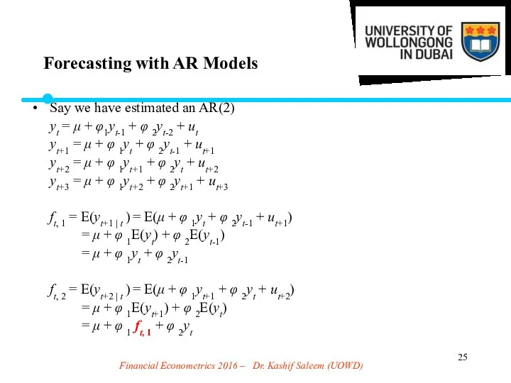
- 25. Financial Econometrics 2016 – Dr. Kashif Saleem (UOWD) Say we have estimated an AR(2) yt =
- 26. Financial Econometrics 2016 – Dr. Kashif Saleem (UOWD) ft, 3 = E(yt+3 | t ) =
- 27. Financial Econometrics 2016 – Dr. Kashif Saleem (UOWD) Some of the most popular criteria for assessing
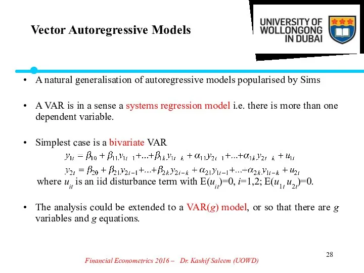
- 28. Financial Econometrics 2016 – Dr. Kashif Saleem (UOWD) A natural generalisation of autoregressive models popularised by
- 29. Financial Econometrics 2016 – Dr. Kashif Saleem (UOWD) One important feature of VARs is the compactness
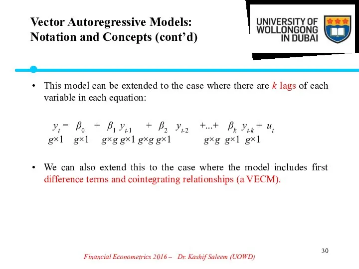
- 30. Financial Econometrics 2016 – Dr. Kashif Saleem (UOWD) This model can be extended to the case
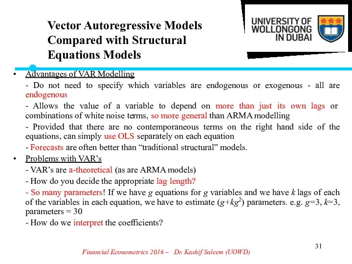
- 31. Financial Econometrics 2016 – Dr. Kashif Saleem (UOWD) Advantages of VAR Modelling - Do not need
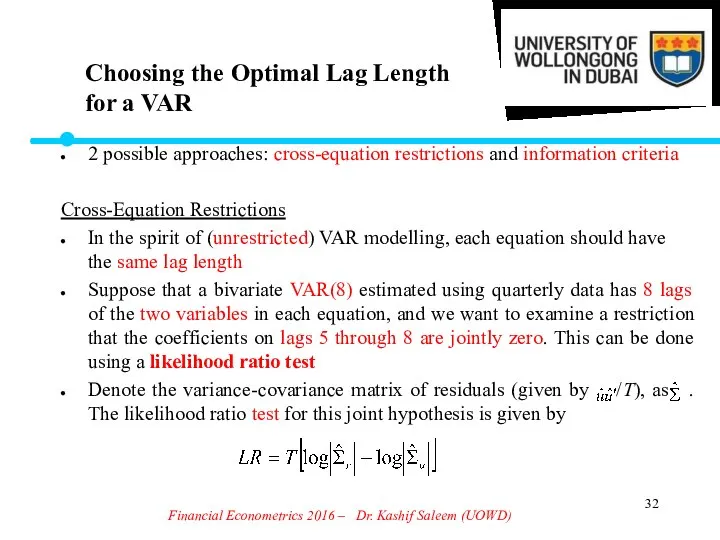
- 32. Financial Econometrics 2016 – Dr. Kashif Saleem (UOWD) Choosing the Optimal Lag Length for a VAR
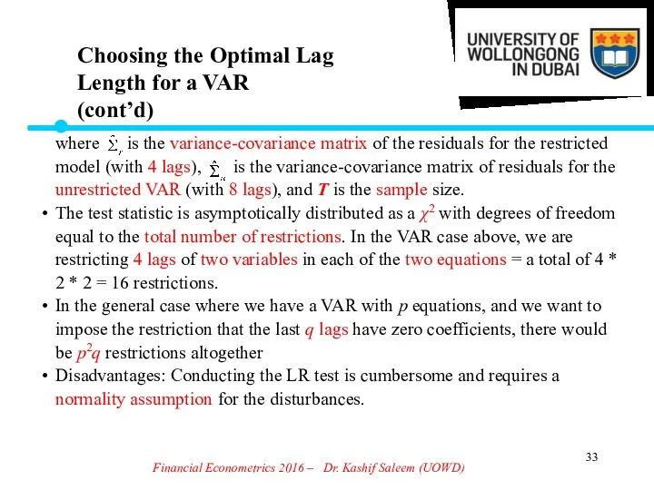
- 33. Financial Econometrics 2016 – Dr. Kashif Saleem (UOWD) Choosing the Optimal Lag Length for a VAR
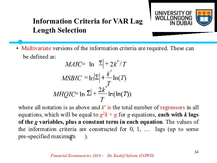
- 34. Financial Econometrics 2016 – Dr. Kashif Saleem (UOWD) Information Criteria for VAR Lag Length Selection Multivariate
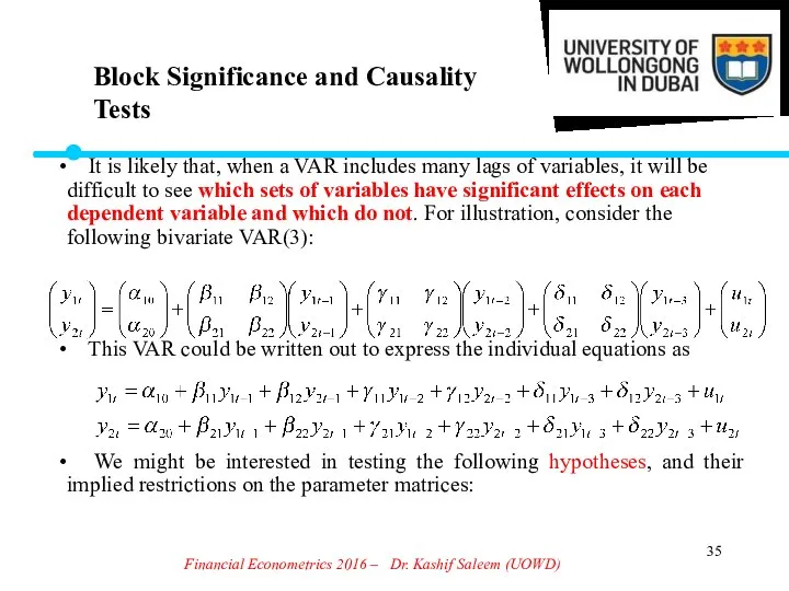
- 35. Financial Econometrics 2016 – Dr. Kashif Saleem (UOWD) Block Significance and Causality Tests It is likely
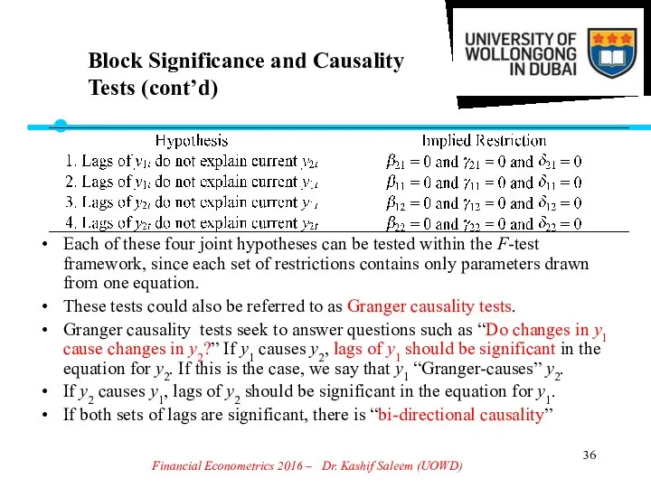
- 36. Financial Econometrics 2016 – Dr. Kashif Saleem (UOWD) Block Significance and Causality Tests (cont’d) Each of
- 37. Financial Econometrics 2016 – Dr. Kashif Saleem (UOWD) Impulse Responses VAR models are often difficult to
- 38. Financial Econometrics 2016 – Dr. Kashif Saleem (UOWD) Variance Decompositions Variance decompositions offer a slightly different
- 39. Home Assignment Vector Autoregressive Model: Run a VAR (3) model by using exchange rate data on
- 41. Скачать презентацию
Financial Econometrics 2016 – Dr. Kashif Saleem (UOWD)
Univariate time series models
Univariate
Financial Econometrics 2016 – Dr. Kashif Saleem (UOWD)
Univariate time series models
Univariate
Quantitative Economic Analysis – 2016, Dr. Kashif Saleem (UOWD)
Let ut (t=1,2,3,...)
Quantitative Economic Analysis – 2016, Dr. Kashif Saleem (UOWD)
Let ut (t=1,2,3,...)
Financial Econometrics 2016 – Dr. Kashif Saleem (UOWD)
An autoregressive model of
Financial Econometrics 2016 – Dr. Kashif Saleem (UOWD)
An autoregressive model of
Financial Econometrics 2016 – Dr. Kashif Saleem (UOWD)
By combining the AR(p)
Financial Econometrics 2016 – Dr. Kashif Saleem (UOWD)
By combining the AR(p)
Financial Econometrics 2016 – Dr. Kashif Saleem (UOWD)
An autoregressive process has
a
Financial Econometrics 2016 – Dr. Kashif Saleem (UOWD)
An autoregressive process has
a
Financial Econometrics 2016 – Dr. Kashif Saleem (UOWD)
The acf and pacf
Financial Econometrics 2016 – Dr. Kashif Saleem (UOWD)
The acf and pacf

Financial Econometrics 2016 – Dr. Kashif Saleem (UOWD)
ACF and PACF for
Financial Econometrics 2016 – Dr. Kashif Saleem (UOWD)
ACF and PACF for
Financial Econometrics 2016 – Dr. Kashif Saleem (UOWD)
ACF and PACF for
Financial Econometrics 2016 – Dr. Kashif Saleem (UOWD)
ACF and PACF for
Financial Econometrics 2016 – Dr. Kashif Saleem (UOWD)
ACF and PACF for
Financial Econometrics 2016 – Dr. Kashif Saleem (UOWD)
ACF and PACF for
Financial Econometrics 2016 – Dr. Kashif Saleem (UOWD)
ACF and PACF for
Financial Econometrics 2016 – Dr. Kashif Saleem (UOWD)
ACF and PACF for
Financial Econometrics 2016 – Dr. Kashif Saleem (UOWD)
ACF and PACF for
Financial Econometrics 2016 – Dr. Kashif Saleem (UOWD)
ACF and PACF for
Financial Econometrics 2016 – Dr. Kashif Saleem (UOWD)
ACF and PACF for
Financial Econometrics 2016 – Dr. Kashif Saleem (UOWD)
ACF and PACF for
Financial Econometrics 2016 – Dr. Kashif Saleem (UOWD)
Box and Jenkins (1970)
Financial Econometrics 2016 – Dr. Kashif Saleem (UOWD)
Box and Jenkins (1970)
Financial Econometrics 2016 – Dr. Kashif Saleem (UOWD)
Step 2:
- Estimation of
Financial Econometrics 2016 – Dr. Kashif Saleem (UOWD)
Step 2:
- Estimation of

Financial Econometrics 2016 – Dr. Kashif Saleem (UOWD)
Identification would typically not
Financial Econometrics 2016 – Dr. Kashif Saleem (UOWD)
Identification would typically not
Financial Econometrics 2016 – Dr. Kashif Saleem (UOWD)
The three most popular
Financial Econometrics 2016 – Dr. Kashif Saleem (UOWD)
The three most popular
Financial Econometrics 2016 – Dr. Kashif Saleem (UOWD)
As distinct from ARMA
Financial Econometrics 2016 – Dr. Kashif Saleem (UOWD)
As distinct from ARMA
Financial Econometrics 2016 – Dr. Kashif Saleem (UOWD)
Another modelling and forecasting
Financial Econometrics 2016 – Dr. Kashif Saleem (UOWD)
Another modelling and forecasting
Financial Econometrics 2016 – Dr. Kashif Saleem (UOWD)
Forecasting = prediction.
An important
Financial Econometrics 2016 – Dr. Kashif Saleem (UOWD)
Forecasting = prediction.
An important
Financial Econometrics 2016 – Dr. Kashif Saleem (UOWD)
Expect the “forecast” of
Financial Econometrics 2016 – Dr. Kashif Saleem (UOWD)
Expect the “forecast” of
Financial Econometrics 2016 – Dr. Kashif Saleem (UOWD)
Models for Forecasting
Financial Econometrics 2016 – Dr. Kashif Saleem (UOWD)
Models for Forecasting
Financial Econometrics 2016 – Dr. Kashif Saleem (UOWD)
An MA(q) only has
Financial Econometrics 2016 – Dr. Kashif Saleem (UOWD)
An MA(q) only has
Financial Econometrics 2016 – Dr. Kashif Saleem (UOWD)
ft, 1 = E(yt+1
Financial Econometrics 2016 – Dr. Kashif Saleem (UOWD)
ft, 1 = E(yt+1
Financial Econometrics 2016 – Dr. Kashif Saleem (UOWD)
Say we have estimated
Financial Econometrics 2016 – Dr. Kashif Saleem (UOWD)
Say we have estimated

Financial Econometrics 2016 – Dr. Kashif Saleem (UOWD)
ft, 3 = E(yt+3
Financial Econometrics 2016 – Dr. Kashif Saleem (UOWD)
ft, 3 = E(yt+3

Financial Econometrics 2016 – Dr. Kashif Saleem (UOWD)
Some of the most
Financial Econometrics 2016 – Dr. Kashif Saleem (UOWD)
Some of the most
Financial Econometrics 2016 – Dr. Kashif Saleem (UOWD)
A natural generalisation of
Financial Econometrics 2016 – Dr. Kashif Saleem (UOWD)
A natural generalisation of

Financial Econometrics 2016 – Dr. Kashif Saleem (UOWD)
One important feature of
Financial Econometrics 2016 – Dr. Kashif Saleem (UOWD)
One important feature of
Financial Econometrics 2016 – Dr. Kashif Saleem (UOWD)
This model can be
Financial Econometrics 2016 – Dr. Kashif Saleem (UOWD)
This model can be
Financial Econometrics 2016 – Dr. Kashif Saleem (UOWD)
Advantages of VAR Modelling
-
Financial Econometrics 2016 – Dr. Kashif Saleem (UOWD)
Advantages of VAR Modelling
-
Financial Econometrics 2016 – Dr. Kashif Saleem (UOWD)
Choosing the Optimal Lag
Financial Econometrics 2016 – Dr. Kashif Saleem (UOWD)
Choosing the Optimal Lag
Financial Econometrics 2016 – Dr. Kashif Saleem (UOWD)
Choosing the Optimal Lag
Financial Econometrics 2016 – Dr. Kashif Saleem (UOWD)
Choosing the Optimal Lag
Financial Econometrics 2016 – Dr. Kashif Saleem (UOWD)
Information Criteria for VAR
Financial Econometrics 2016 – Dr. Kashif Saleem (UOWD)
Information Criteria for VAR
Financial Econometrics 2016 – Dr. Kashif Saleem (UOWD)
Block Significance and Causality
Financial Econometrics 2016 – Dr. Kashif Saleem (UOWD)
Block Significance and Causality
Financial Econometrics 2016 – Dr. Kashif Saleem (UOWD)
Block Significance and Causality
Financial Econometrics 2016 – Dr. Kashif Saleem (UOWD)
Block Significance and Causality

Financial Econometrics 2016 – Dr. Kashif Saleem (UOWD)
Impulse Responses
VAR models are
Financial Econometrics 2016 – Dr. Kashif Saleem (UOWD)
Impulse Responses
VAR models are
Financial Econometrics 2016 – Dr. Kashif Saleem (UOWD)
Variance Decompositions
Variance decompositions
Financial Econometrics 2016 – Dr. Kashif Saleem (UOWD)
Variance Decompositions
Variance decompositions
Home Assignment
Vector Autoregressive Model:
Run a VAR (3) model by using
Home Assignment
Vector Autoregressive Model:
Run a VAR (3) model by using
 Экономические системы
 Стратегия и тактика ценообразования
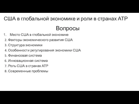 США в глобальной экономике и роли в странах АТР
 Этапы развития экономической науки
 Международные экономические организации
 Экономическая безопасность России
 Типология рынков
 Лекция № 5. Вмешательство государства и общественное благосостояние
 Натуральное хозяйство. Товарное производство
 Экономический механизм возникновения кризисных явлений в деятельности организации
 Презентация Функционалистская теория происхождения культуры
 Предложение инвестиционного фонда Pinnacle Absolute Return Global Alpha Fund
 Мировая экономика
 Меркантилизм и физиократия
 Экономические задачи ЕГЭ
 Коррупция – экономико-правовое обоснование
 Резервы и пути повышения рентабельности машиностроительного предприятия
 Taiwan’s economic situation
 Спрос, предложение и рыночное равновесие
 Потребности, блага, экономический выбор
 Теория систем и системный анализ в экономике. Социально-экономические системы
 Финансовая грамотность и ее проецирование на профессиональную деятельность
 Analiza strategiei de dezvoltare a turismului în România și Rep.Moldova
 Class 4 The Ownership of Nature Objects and Natural Resources
 Социальная политика государства. Политика доходов. Экономика домашнего хозяйства, семьи
 Экономика: наука и хозяйство
 Рынок инноваций
 Основные понятия теории экономики и управления безопасностью