- Deep belief nets

Содержание
- 2. Some things you will learn in this tutorial How to learn multi-layer generative models of unlabelled
- 3. A spectrum of machine learning tasks Low-dimensional data (e.g. less than 100 dimensions) Lots of noise
- 4. Historical background: First generation neural networks Perceptrons (~1960) used a layer of hand-coded features and tried
- 5. Second generation neural networks (~1985) input vector hidden layers outputs Back-propagate error signal to get derivatives
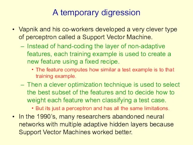
- 6. A temporary digression Vapnik and his co-workers developed a very clever type of perceptron called a
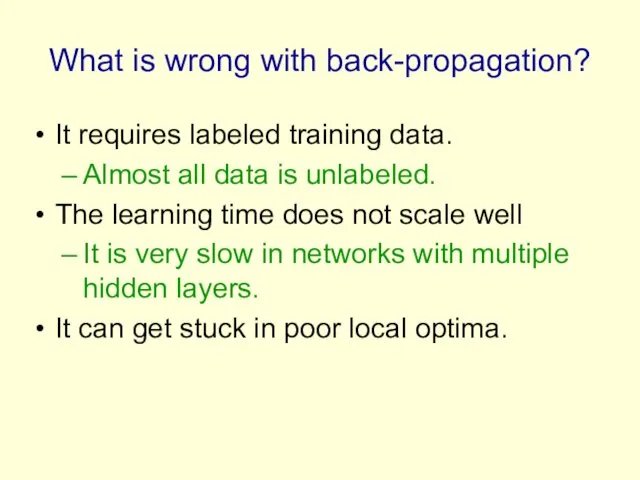
- 7. What is wrong with back-propagation? It requires labeled training data. Almost all data is unlabeled. The
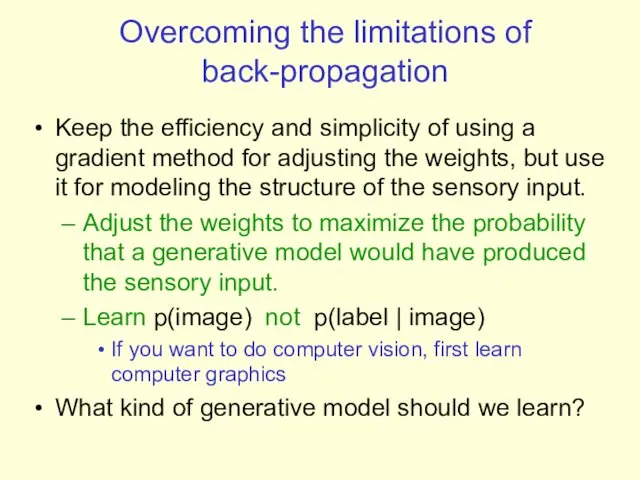
- 8. Overcoming the limitations of back-propagation Keep the efficiency and simplicity of using a gradient method for
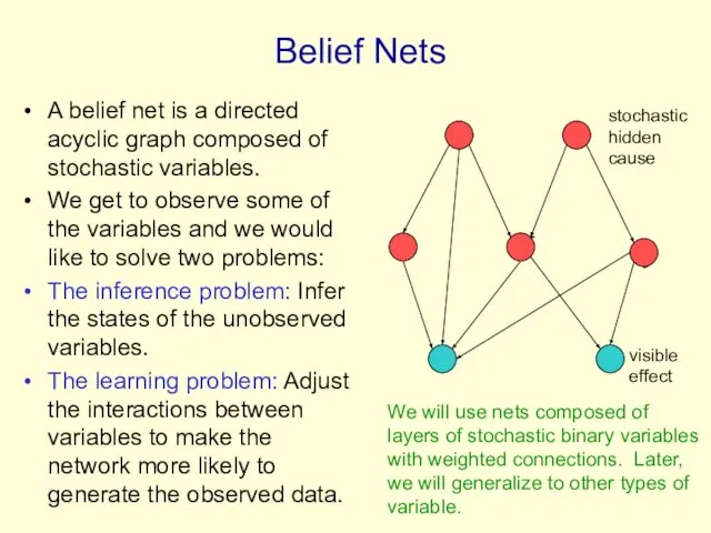
- 9. Belief Nets A belief net is a directed acyclic graph composed of stochastic variables. We get
- 10. Stochastic binary units (Bernoulli variables) These have a state of 1 or 0. The probability of
- 11. Learning Deep Belief Nets It is easy to generate an unbiased example at the leaf nodes,
- 12. The learning rule for sigmoid belief nets Learning is easy if we can get an unbiased
- 13. Explaining away (Judea Pearl) Even if two hidden causes are independent, they can become dependent when
- 14. Why it is usually very hard to learn sigmoid belief nets one layer at a time
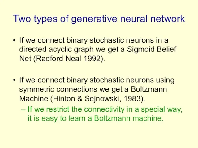
- 15. Two types of generative neural network If we connect binary stochastic neurons in a directed acyclic
- 16. Restricted Boltzmann Machines (Smolensky ,1986, called them “harmoniums”) We restrict the connectivity to make learning easier.
- 17. The Energy of a joint configuration (ignoring terms to do with biases) weight between units i
- 18. Weights ? Energies ? Probabilities Each possible joint configuration of the visible and hidden units has
- 19. Using energies to define probabilities The probability of a joint configuration over both visible and hidden
- 20. A picture of the maximum likelihood learning algorithm for an RBM i j i j i
- 21. A quick way to learn an RBM i j i j t = 0 t =
- 22. How to learn a set of features that are good for reconstructing images of the digit
- 23. The final 50 x 256 weights Each neuron grabs a different feature.
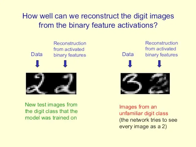
- 24. Reconstruction from activated binary features Data Reconstruction from activated binary features Data How well can we
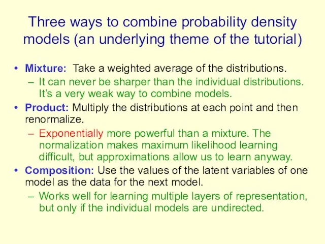
- 25. Three ways to combine probability density models (an underlying theme of the tutorial) Mixture: Take a
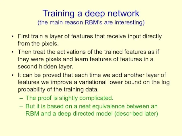
- 26. Training a deep network (the main reason RBM’s are interesting) First train a layer of features
- 27. The generative model after learning 3 layers To generate data: Get an equilibrium sample from the
- 28. Why does greedy learning work? An aside: Averaging factorial distributions If you average some factorial distributions,
- 29. Why does greedy learning work? Each RBM converts its data distribution into an aggregated posterior distribution
- 30. Why does greedy learning work? The weights, W, in the bottom level RBM define p(v|h) and
- 31. Which distributions are factorial in a directed belief net? In a directed belief net with one
- 32. Why does greedy learning fail in a directed module? A directed module also converts its data
- 33. A model of digit recognition 2000 top-level neurons 500 neurons 500 neurons 28 x 28 pixel
- 34. Fine-tuning with a contrastive version of the “wake-sleep” algorithm After learning many layers of features, we
- 35. Show the movie of the network generating digits (available at www.cs.toronto/~hinton)
- 36. Samples generated by letting the associative memory run with one label clamped. There are 1000 iterations
- 37. Examples of correctly recognized handwritten digits that the neural network had never seen before Its very
- 38. How well does it discriminate on MNIST test set with no extra information about geometric distortions?
- 39. Unsupervised “pre-training” also helps for models that have more data and better priors Ranzato et. al.
- 40. Another view of why layer-by-layer learning works There is an unexpected equivalence between RBM’s and directed
- 41. An infinite sigmoid belief net that is equivalent to an RBM The distribution generated by this
- 42. The variables in h0 are conditionally independent given v0. Inference is trivial. We just multiply v0
- 43. The learning rule for a sigmoid belief net is: With replicated weights this becomes: v1 h1
- 44. First learn with all the weights tied This is exactly equivalent to learning an RBM Contrastive
- 45. Then freeze the first layer of weights in both directions and learn the remaining weights (still
- 46. How many layers should we use and how wide should they be? (I am indebted to
- 47. What happens when the weights in higher layers become different from the weights in the first
- 48. A stack of RBM’s (Yee-Whye Teh’s idea) Each RBM has the same subscript as its hidden
- 49. The variational bound Now we cancel out all of the partition functions except the top one
- 50. Summary so far Restricted Boltzmann Machines provide a simple way to learn a layer of features
- 51. Overview of the rest of the tutorial How to fine-tune a greedily trained generative model to
- 52. BREAK
- 53. Fine-tuning for discrimination First learn one layer at a time greedily. Then treat this as “pre-training”
- 54. Why backpropagation works better after greedy pre-training Greedily learning one layer at a time scales well
- 55. First, model the distribution of digit images 2000 units 500 units 500 units 28 x 28
- 56. Results on permutation-invariant MNIST task Very carefully trained backprop net with 1.6% one or two hidden
- 57. Combining deep belief nets with Gaussian processes Deep belief nets can benefit a lot from unlabeled
- 58. Learning to extract the orientation of a face patch (Salakhutdinov & Hinton, NIPS 2007)
- 59. The training and test sets 11,000 unlabeled cases 100, 500, or 1000 labeled cases face patches
- 60. The root mean squared error in the orientation when combining GP’s with deep belief nets 22.2
- 61. Modeling real-valued data For images of digits it is possible to represent intermediate intensities as if
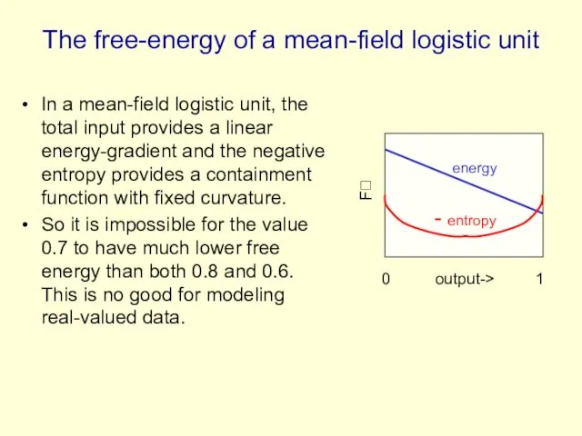
- 62. The free-energy of a mean-field logistic unit In a mean-field logistic unit, the total input provides
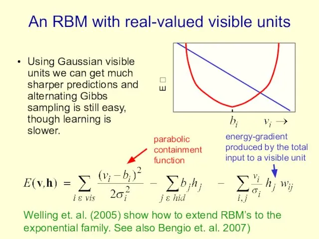
- 63. An RBM with real-valued visible units Using Gaussian visible units we can get much sharper predictions
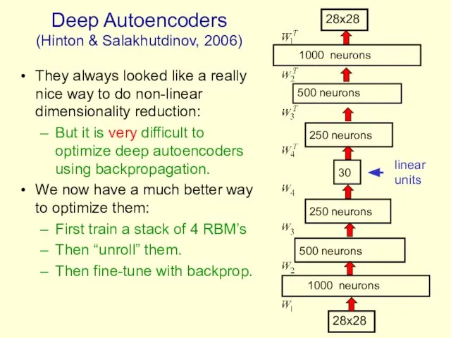
- 64. Deep Autoencoders (Hinton & Salakhutdinov, 2006) They always looked like a really nice way to do
- 65. A comparison of methods for compressing digit images to 30 real numbers. real data 30-D deep
- 66. Do the 30-D codes found by the deep autoencoder preserve the class structure of the data?
- 67. entirely unsupervised except for the colors
- 68. Retrieving documents that are similar to a query document We can use an autoencoder to find
- 69. How to compress the count vector We train the neural network to reproduce its input vector
- 70. Performance of the autoencoder at document retrieval Train on bags of 2000 words for 400,000 training
- 71. Proportion of retrieved documents in same class as query Number of documents retrieved
- 72. First compress all documents to 2 numbers using a type of PCA Then use different colors
- 73. First compress all documents to 2 numbers. Then use different colors for different document categories
- 74. Finding binary codes for documents Train an auto-encoder using 30 logistic units for the code layer.
- 75. Semantic hashing: Using a deep autoencoder as a hash-function for finding approximate matches (Salakhutdinov & Hinton,
- 76. How good is a shortlist found this way? We have only implemented it for a million
- 77. Time series models Inference is difficult in directed models of time series if we use non-linear
- 78. Time series models If we really need distributed representations (which we nearly always do), we can
- 79. The conditional RBM model (Sutskever & Hinton 2007) Given the data and the previous hidden state,
- 80. Why the autoregressive connections do not cause problems The autoregressive connections do not mess up contrastive
- 81. Generating from a learned model The inputs from the earlier states of the visible units create
- 82. Stacking temporal RBM’s Treat the hidden activities of the first level TRBM as the data for
- 83. An application to modeling motion capture data (Taylor, Roweis & Hinton, 2007) Human motion can be
- 84. Modeling multiple types of motion We can easily learn to model walking and running in a
- 85. Show Graham Taylor’s movies available at www.cs.toronto/~hinton
- 86. Generating the parts of an object One way to maintain the constraints between the parts is
- 87. Semi-restricted Boltzmann Machines We restrict the connectivity to make learning easier. Contrastive divergence learning requires the
- 88. Learning a semi-restricted Boltzmann Machine i j i j t = 0 t = 1 1.
- 89. Learning in Semi-restricted Boltzmann Machines Method 1: To form a reconstruction, cycle through the visible units
- 90. Results on modeling natural image patches using a stack of RBM’s (Osindero and Hinton) Stack of
- 91. Without lateral connections real data samples from model
- 92. With lateral connections real data samples from model
- 93. A funny way to use an MRF The lateral connections form an MRF. The MRF is
- 94. Why do we whiten data? Images typically have strong pair-wise correlations. Learning higher order statistics is
- 95. Whitening the learning signal instead of the data Contrastive divergence learning can remove the effects of
- 96. Towards a more powerful, multi-linear stackable learning module So far, the states of the units in
- 97. Higher order Boltzmann machines (Sejnowski, ~1986) The usual energy function is quadratic in the states: But
- 98. A picture of a conditional, higher-order Boltzmann machine (Hinton & Lang,1985) retina-based features object-based features viewing
- 99. Using conditional higher-order Boltzmann machines to model image transformations (Memisevic and Hinton, 2007) A transformation unit
- 101. Скачать презентацию
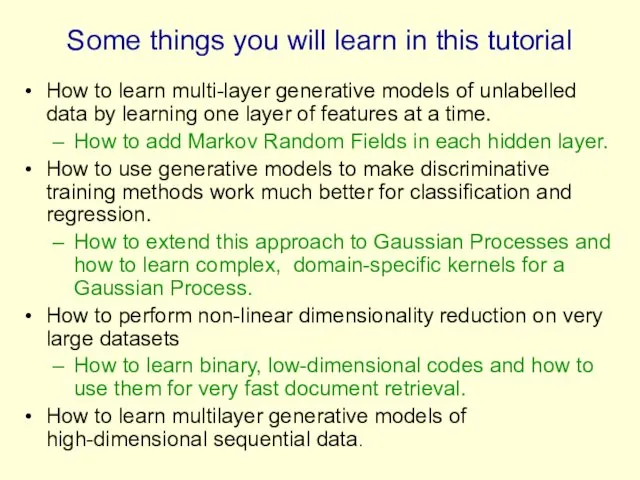
Some things you will learn in this tutorial
How to learn multi-layer
Some things you will learn in this tutorial
How to learn multi-layer
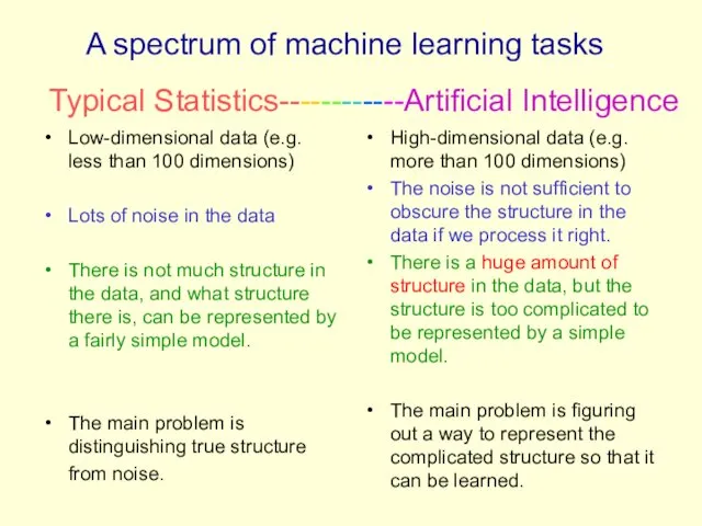
A spectrum of machine learning tasks
Low-dimensional data (e.g. less than 100
A spectrum of machine learning tasks
Low-dimensional data (e.g. less than 100
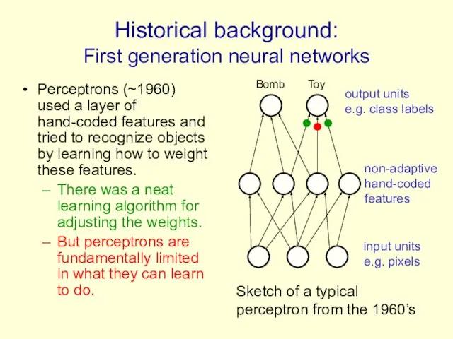
Historical background:
First generation neural networks
Perceptrons (~1960) used a layer of hand-coded
Historical background:
First generation neural networks
Perceptrons (~1960) used a layer of hand-coded
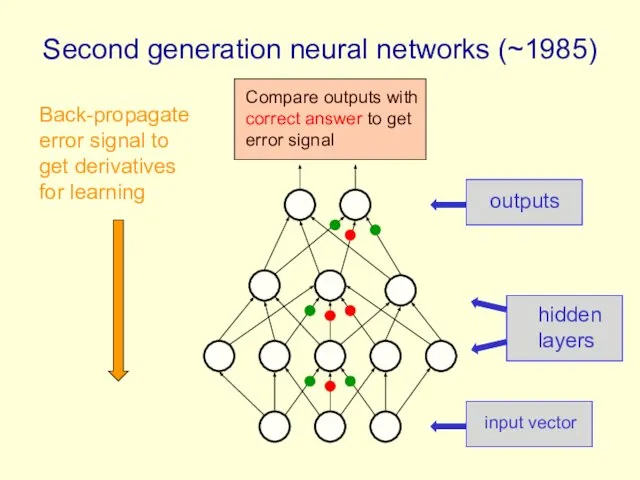
Second generation neural networks (~1985)
input vector
hidden layers
outputs
Back-propagate error signal to get
Second generation neural networks (~1985)
input vector
hidden layers
outputs
Back-propagate error signal to get
A temporary digression
Vapnik and his co-workers developed a very clever type
A temporary digression
Vapnik and his co-workers developed a very clever type
What is wrong with back-propagation?
It requires labeled training data.
Almost all data
What is wrong with back-propagation?
It requires labeled training data.
Almost all data
Overcoming the limitations of back-propagation
Keep the efficiency and simplicity of using
Overcoming the limitations of back-propagation
Keep the efficiency and simplicity of using
Belief Nets
A belief net is a directed acyclic graph composed
Belief Nets
A belief net is a directed acyclic graph composed
Stochastic binary units
(Bernoulli variables)
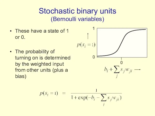
These have a state of 1 or 0.
The
Stochastic binary units
(Bernoulli variables)
These have a state of 1 or 0.
The
Learning Deep Belief Nets
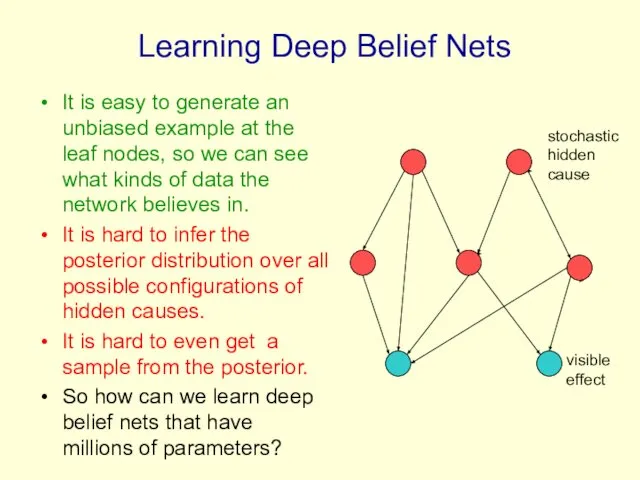
It is easy to generate an unbiased
Learning Deep Belief Nets
It is easy to generate an unbiased
The learning rule for sigmoid belief nets
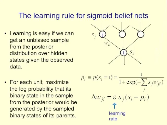
Learning is easy if we
The learning rule for sigmoid belief nets
Learning is easy if we
Explaining away (Judea Pearl)
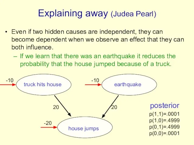
Even if two hidden causes are independent, they
Explaining away (Judea Pearl)
Even if two hidden causes are independent, they
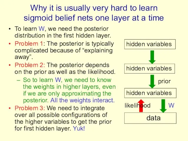
Why it is usually very hard to learn sigmoid belief nets
Why it is usually very hard to learn sigmoid belief nets
Two types of generative neural network
If we connect binary stochastic neurons
Two types of generative neural network
If we connect binary stochastic neurons
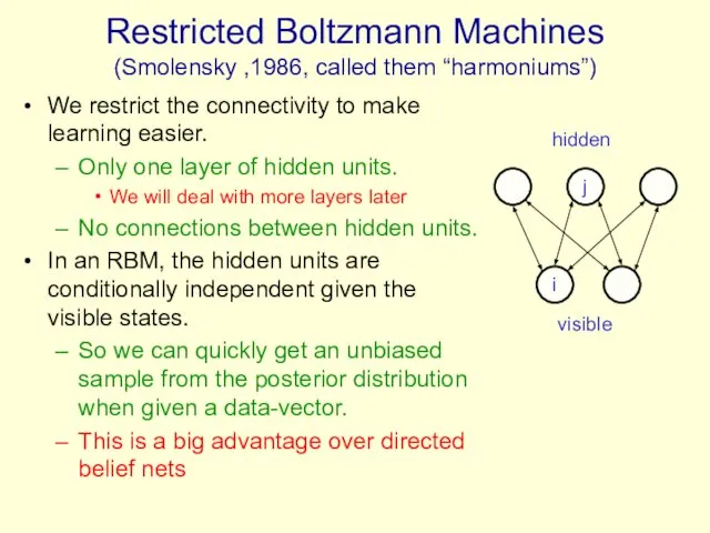
Restricted Boltzmann Machines
(Smolensky ,1986, called them “harmoniums”)
We restrict the connectivity to
Restricted Boltzmann Machines
(Smolensky ,1986, called them “harmoniums”)
We restrict the connectivity to
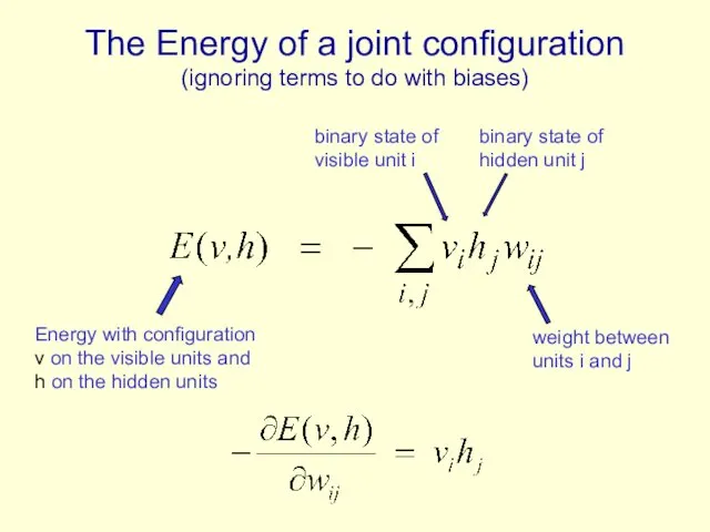
The Energy of a joint configuration
(ignoring terms to do with biases)
weight
The Energy of a joint configuration
(ignoring terms to do with biases)
weight
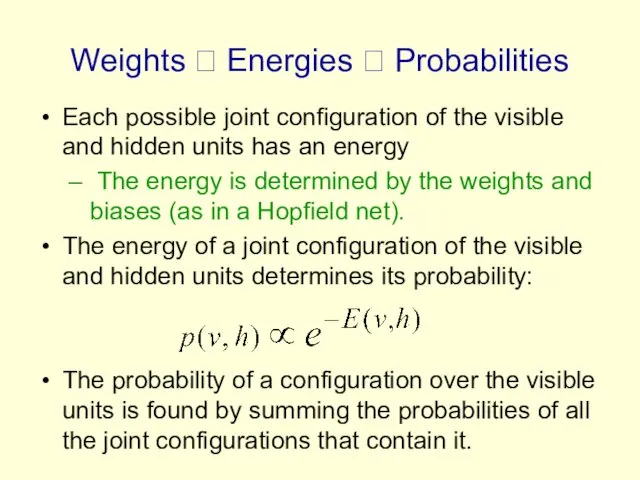
Weights ? Energies ? Probabilities
Each possible joint configuration of the visible
Weights ? Energies ? Probabilities
Each possible joint configuration of the visible
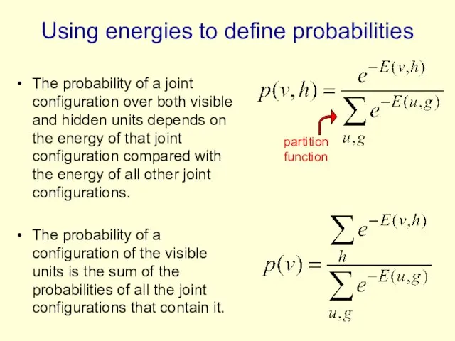
Using energies to define probabilities
The probability of a joint configuration over
Using energies to define probabilities
The probability of a joint configuration over
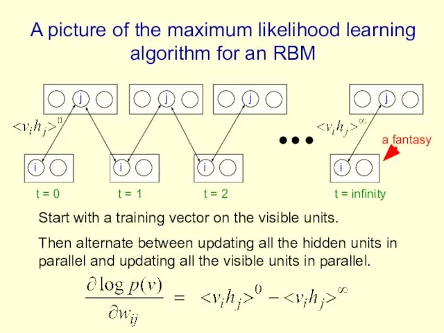
A picture of the maximum likelihood learning algorithm for an RBM
i
j
i
j
i
j
i
j
t
A picture of the maximum likelihood learning algorithm for an RBM
i
j
i
j
i
j
i
j
t
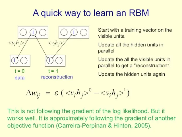
A quick way to learn an RBM
i
j
i
j
t = 0 t =
A quick way to learn an RBM
i
j
i
j
t = 0 t =
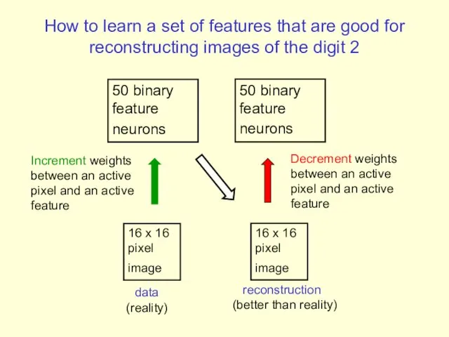
How to learn a set of features that are good for
How to learn a set of features that are good for
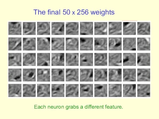
The final 50 x 256 weights
Each neuron grabs a different feature.
The final 50 x 256 weights
Each neuron grabs a different feature.
Reconstruction from activated binary features
Data
Reconstruction from activated binary features
Data
How well can
Reconstruction from activated binary features
Data
Reconstruction from activated binary features
Data
How well can
Three ways to combine probability density models (an underlying theme of
Three ways to combine probability density models (an underlying theme of
Training a deep network
(the main reason RBM’s are interesting)
First train a
Training a deep network
(the main reason RBM’s are interesting)
First train a
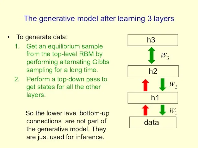
The generative model after learning 3 layers
To generate data:
Get an
The generative model after learning 3 layers
To generate data:
Get an
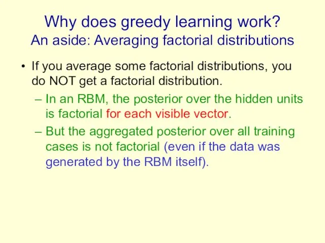
Why does greedy learning work? An aside: Averaging factorial distributions
If
Why does greedy learning work? An aside: Averaging factorial distributions
If
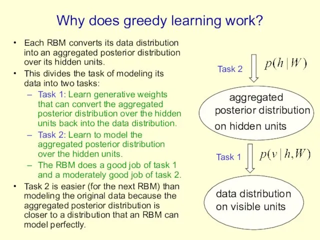
Why does greedy learning work?
Each RBM converts its data distribution into
Why does greedy learning work?
Each RBM converts its data distribution into
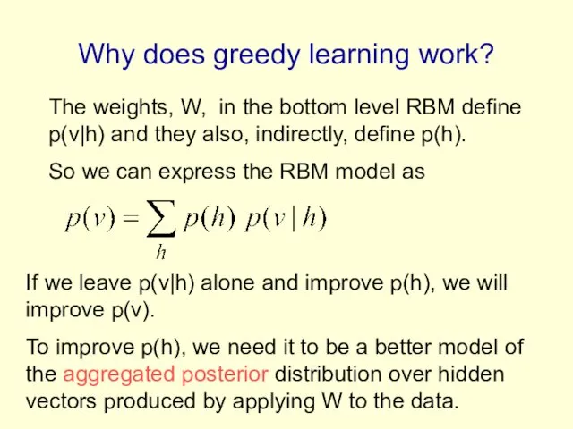
Why does greedy learning work?
The weights, W, in the bottom level
Why does greedy learning work?
The weights, W, in the bottom level
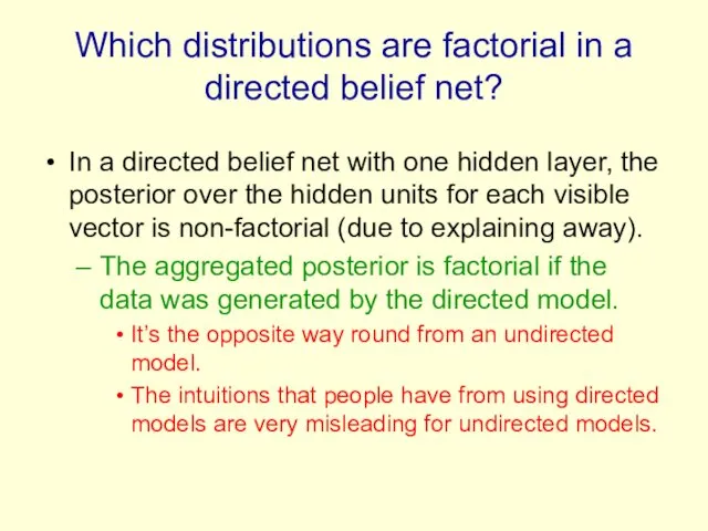
Which distributions are factorial in a directed belief net?
In a directed
Which distributions are factorial in a directed belief net?
In a directed
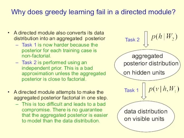
Why does greedy learning fail in a directed module?
A directed module
Why does greedy learning fail in a directed module?
A directed module
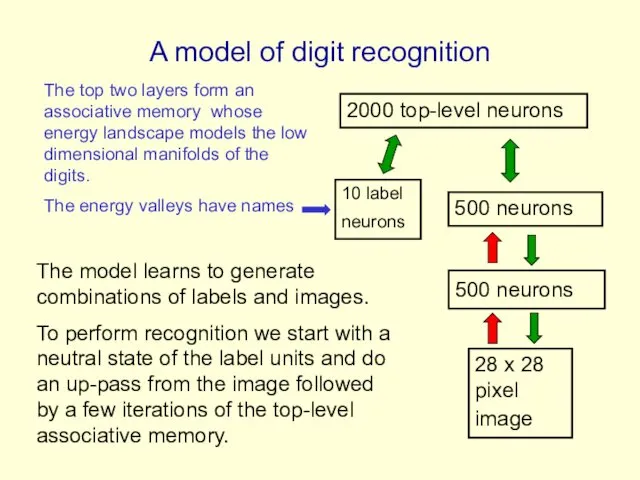
A model of digit recognition
2000 top-level neurons
500 neurons
500 neurons
28 x
A model of digit recognition
2000 top-level neurons
500 neurons
500 neurons
28 x
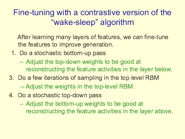
Fine-tuning with a contrastive version of the “wake-sleep” algorithm
After learning
Fine-tuning with a contrastive version of the “wake-sleep” algorithm
After learning

Show the movie of the network generating digits
(available at www.cs.toronto/~hinton)
Show the movie of the network generating digits
(available at www.cs.toronto/~hinton)
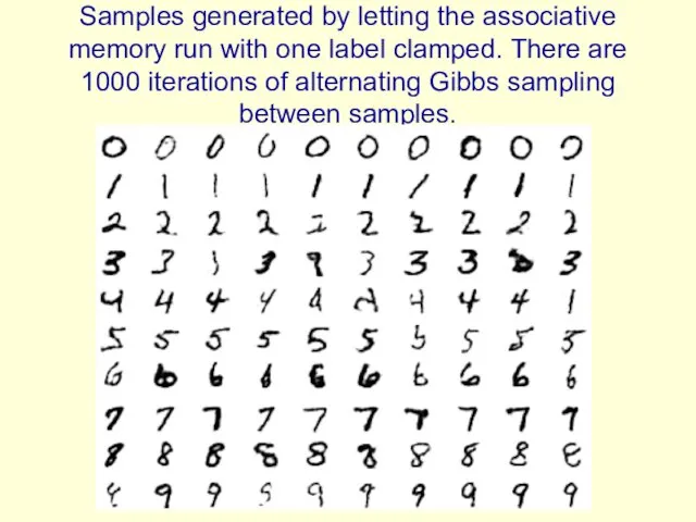
Samples generated by letting the associative memory run with one label
Samples generated by letting the associative memory run with one label
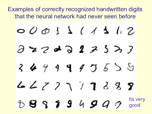
Examples of correctly recognized handwritten digits
that the neural network had never
Examples of correctly recognized handwritten digits that the neural network had never
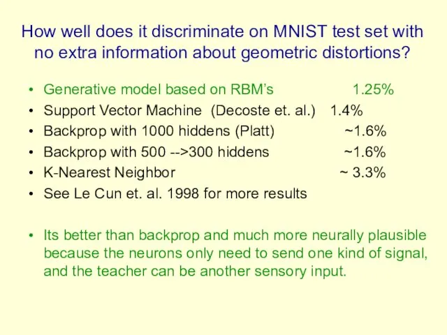
How well does it discriminate on MNIST test set with no
How well does it discriminate on MNIST test set with no
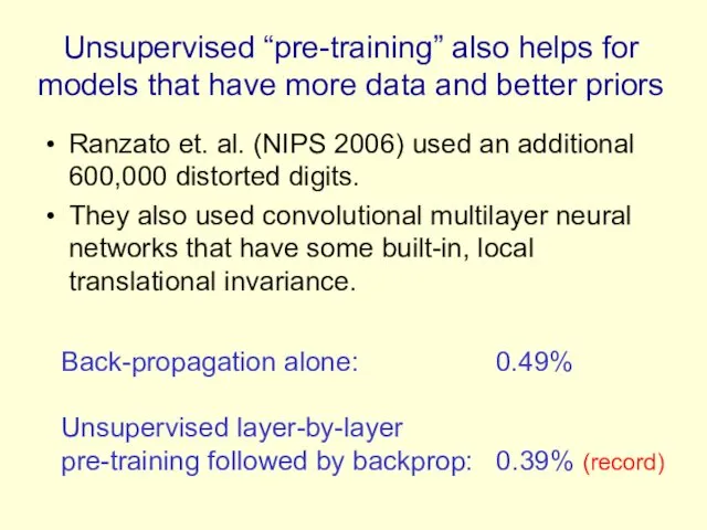
Unsupervised “pre-training” also helps for models that have more data and
Unsupervised “pre-training” also helps for models that have more data and
Another view of why layer-by-layer learning works
There is an unexpected equivalence
Another view of why layer-by-layer learning works
There is an unexpected equivalence
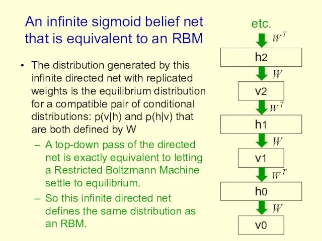
An infinite sigmoid belief net that is equivalent to an RBM
The
An infinite sigmoid belief net that is equivalent to an RBM
The
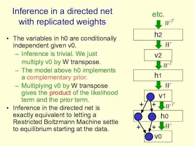
The variables in h0 are conditionally independent given v0.
Inference is trivial.
The variables in h0 are conditionally independent given v0.
Inference is trivial.
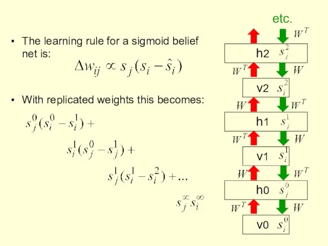
The learning rule for a sigmoid belief net is:
With replicated weights
The learning rule for a sigmoid belief net is:
With replicated weights
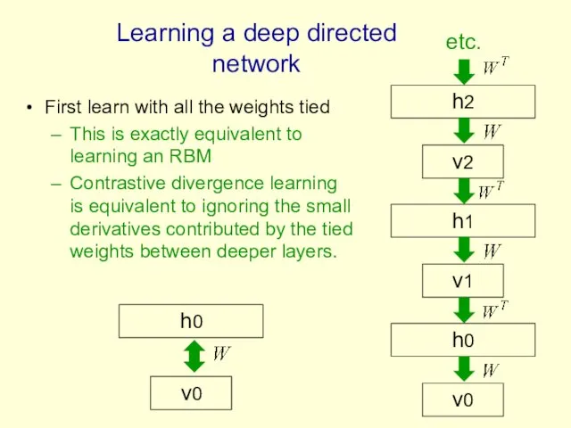
First learn with all the weights tied
This is exactly equivalent to
First learn with all the weights tied
This is exactly equivalent to
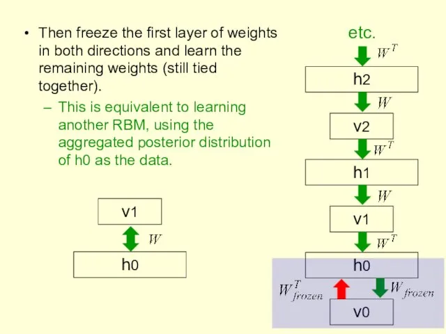
Then freeze the first layer of weights in both directions and
Then freeze the first layer of weights in both directions and
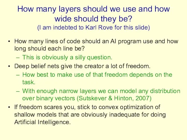
How many layers should we use and how wide should they
How many layers should we use and how wide should they
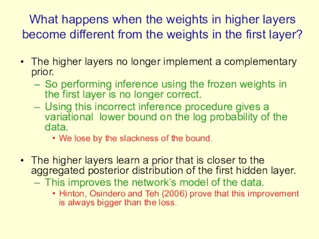
What happens when the weights in higher layers become different from
What happens when the weights in higher layers become different from
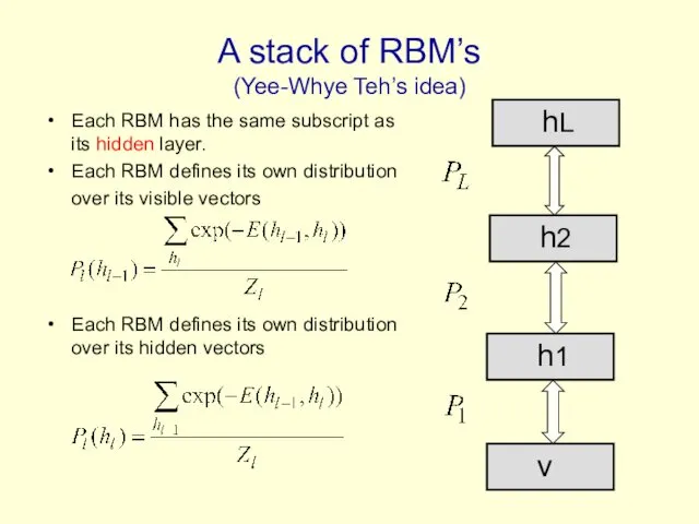
A stack of RBM’s
(Yee-Whye Teh’s idea)
Each RBM has the same subscript
A stack of RBM’s
(Yee-Whye Teh’s idea)
Each RBM has the same subscript
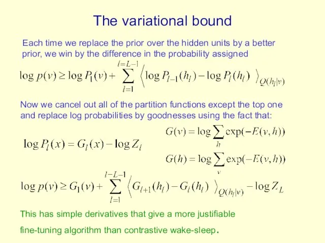
The variational bound
Now we cancel out all of the partition functions
The variational bound
Now we cancel out all of the partition functions
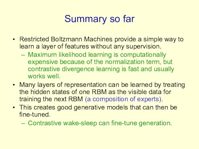
Summary so far
Restricted Boltzmann Machines provide a simple way to learn
Summary so far
Restricted Boltzmann Machines provide a simple way to learn
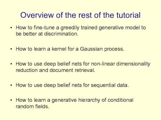
Overview of the rest of the tutorial
How to fine-tune a greedily
Overview of the rest of the tutorial
How to fine-tune a greedily

BREAK
BREAK
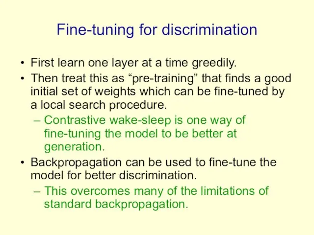
Fine-tuning for discrimination
First learn one layer at a time greedily.
Then treat
Fine-tuning for discrimination
First learn one layer at a time greedily.
Then treat
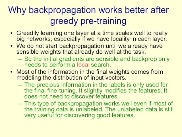
Why backpropagation works better after greedy pre-training
Greedily learning one layer at
Why backpropagation works better after greedy pre-training
Greedily learning one layer at
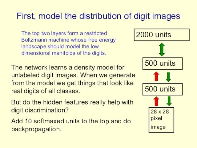
First, model the distribution of digit images
2000 units
500 units
500 units
First, model the distribution of digit images
2000 units
500 units
500 units
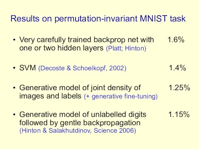
Results on permutation-invariant MNIST task
Very carefully trained backprop net with 1.6%
Results on permutation-invariant MNIST task
Very carefully trained backprop net with 1.6%
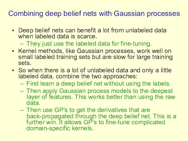
Combining deep belief nets with Gaussian processes
Deep belief nets can benefit
Combining deep belief nets with Gaussian processes
Deep belief nets can benefit
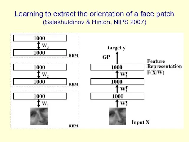
Learning to extract the orientation of a face patch (Salakhutdinov &
Learning to extract the orientation of a face patch (Salakhutdinov &
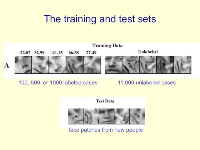
The training and test sets
11,000 unlabeled cases
100, 500, or 1000 labeled
The training and test sets
11,000 unlabeled cases
100, 500, or 1000 labeled
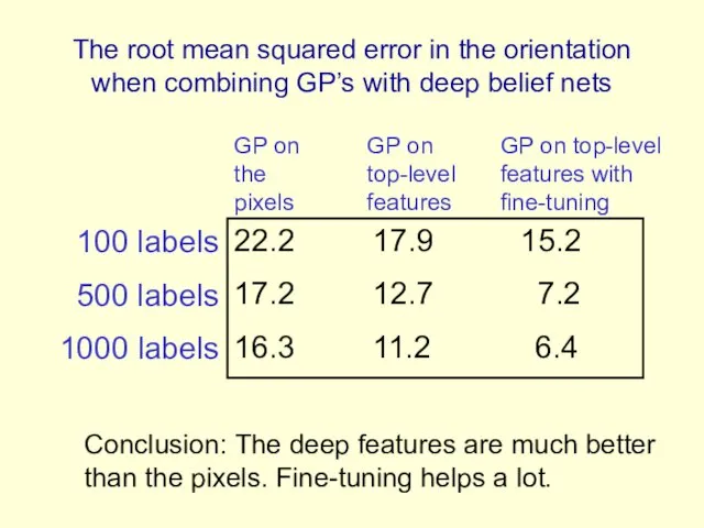
The root mean squared error in the orientation when combining GP’s
The root mean squared error in the orientation when combining GP’s
Modeling real-valued data
For images of digits it is possible to represent
Modeling real-valued data
For images of digits it is possible to represent
The free-energy of a mean-field logistic unit
In a mean-field logistic unit,
The free-energy of a mean-field logistic unit
In a mean-field logistic unit,
An RBM with real-valued visible units
Using Gaussian visible units we can
An RBM with real-valued visible units
Using Gaussian visible units we can
Deep Autoencoders
(Hinton & Salakhutdinov, 2006)
They always looked like a really nice
Deep Autoencoders
(Hinton & Salakhutdinov, 2006)
They always looked like a really nice
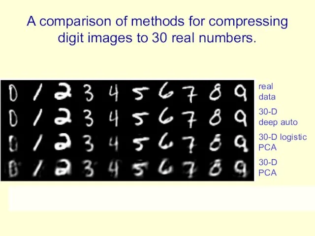
A comparison of methods for compressing digit images to 30 real
A comparison of methods for compressing digit images to 30 real
Do the 30-D codes found by the deep autoencoder preserve the
Do the 30-D codes found by the deep autoencoder preserve the
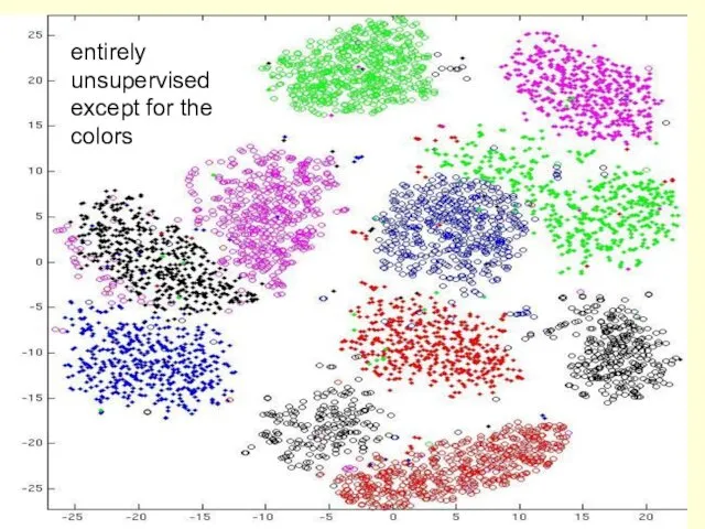
entirely unsupervised except for the colors
entirely unsupervised except for the colors
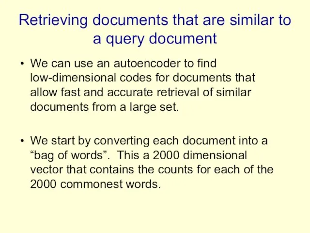
Retrieving documents that are similar to a query document
We can use
Retrieving documents that are similar to a query document
We can use
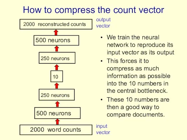
How to compress the count vector
We train the neural network
How to compress the count vector
We train the neural network
Performance of the autoencoder at document retrieval
Train on bags of 2000
Performance of the autoencoder at document retrieval
Train on bags of 2000
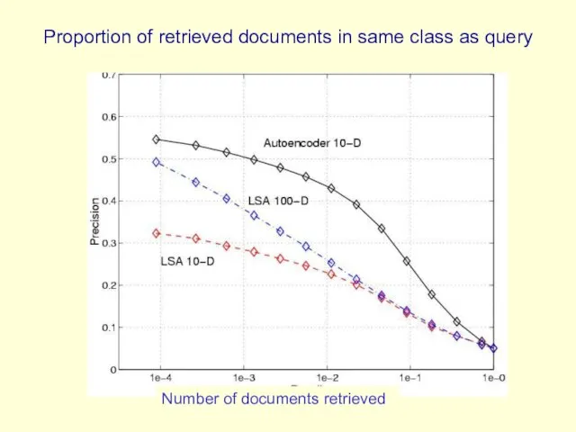
Proportion of retrieved documents in same class as query
Number of documents
Proportion of retrieved documents in same class as query
Number of documents
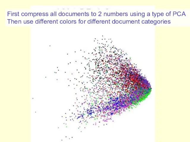
First compress all documents to 2 numbers using a type of
First compress all documents to 2 numbers using a type of
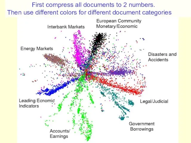
First compress all documents to 2 numbers. Then use different
First compress all documents to 2 numbers. Then use different
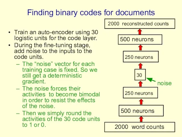
Finding binary codes for documents
Train an auto-encoder using 30 logistic units
Finding binary codes for documents
Train an auto-encoder using 30 logistic units
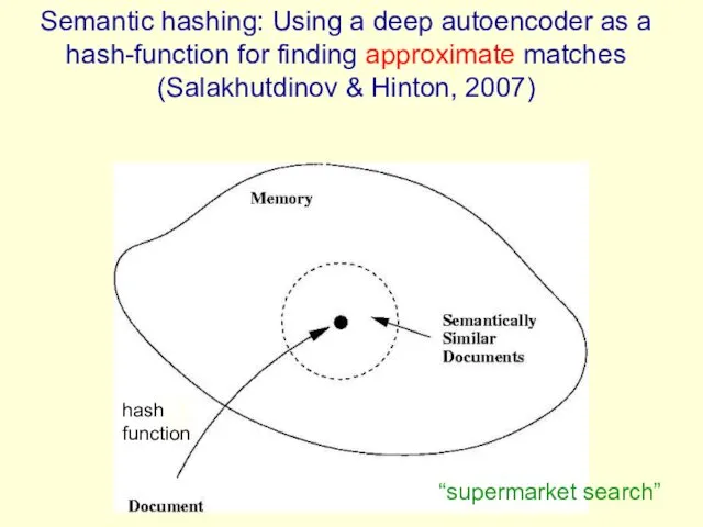
Semantic hashing: Using a deep autoencoder as a hash-function for finding
Semantic hashing: Using a deep autoencoder as a hash-function for finding
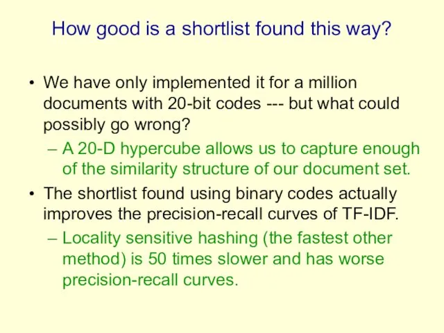
How good is a shortlist found this way?
We have only
How good is a shortlist found this way?
We have only
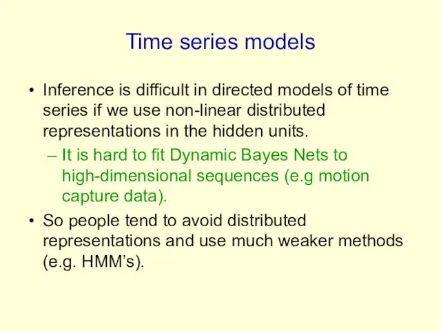
Time series models
Inference is difficult in directed models of time series
Time series models
Inference is difficult in directed models of time series
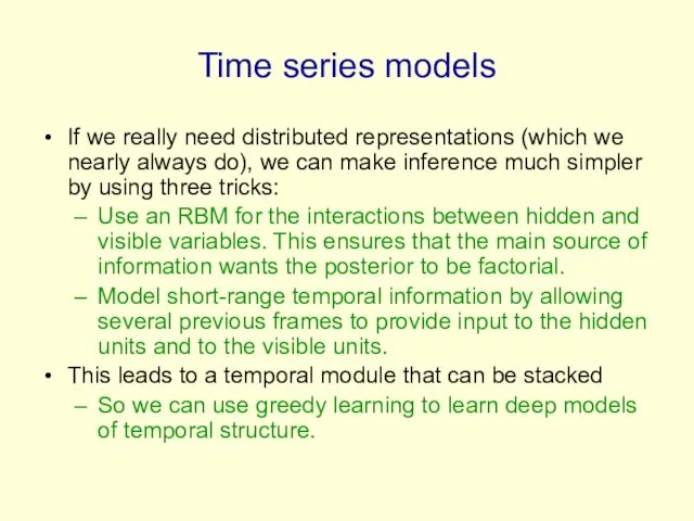
Time series models
If we really need distributed representations (which we nearly
Time series models
If we really need distributed representations (which we nearly
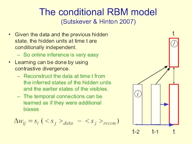
The conditional RBM model
(Sutskever & Hinton 2007)
Given the data and
The conditional RBM model
(Sutskever & Hinton 2007)
Given the data and
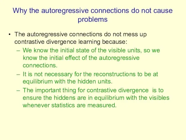
Why the autoregressive connections do not cause problems
The autoregressive connections do
Why the autoregressive connections do not cause problems
The autoregressive connections do
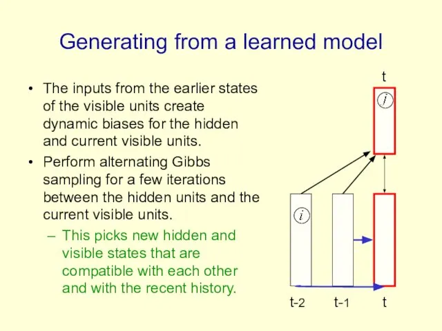
Generating from a learned model
The inputs from the earlier states of
Generating from a learned model
The inputs from the earlier states of
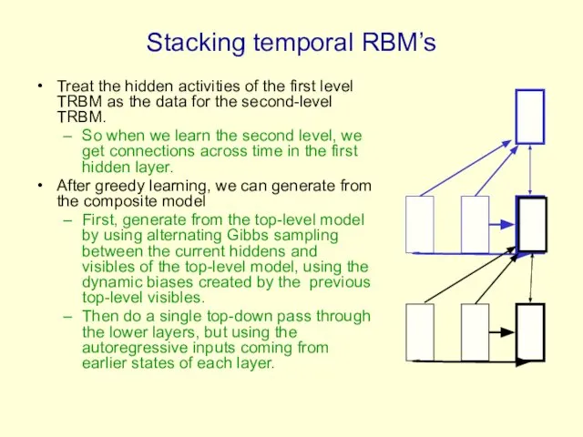
Stacking temporal RBM’s
Treat the hidden activities of the first level TRBM
Stacking temporal RBM’s
Treat the hidden activities of the first level TRBM
An application to modeling
motion capture data
(Taylor, Roweis & Hinton,
An application to modeling motion capture data (Taylor, Roweis & Hinton,
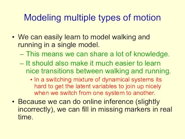
Modeling multiple types of motion
We can easily learn to model walking
Modeling multiple types of motion
We can easily learn to model walking

Show Graham Taylor’s movies
available at www.cs.toronto/~hinton
Show Graham Taylor’s movies
available at www.cs.toronto/~hinton
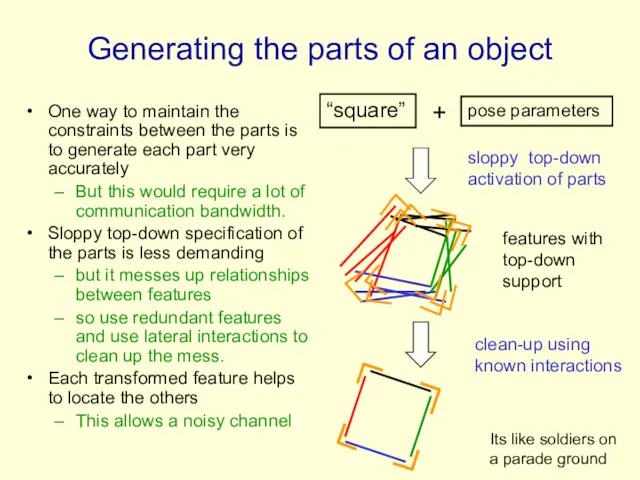
Generating the parts of an object
One way to maintain the
Generating the parts of an object
One way to maintain the
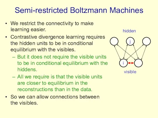
Semi-restricted Boltzmann Machines
We restrict the connectivity to make learning easier.
Contrastive divergence
Semi-restricted Boltzmann Machines
We restrict the connectivity to make learning easier.
Contrastive divergence
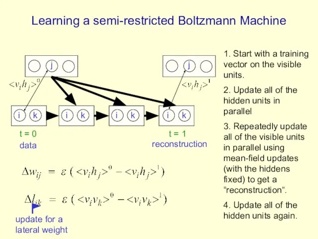
Learning a semi-restricted Boltzmann Machine
i
j
i
j
t = 0 t = 1
1.
Learning a semi-restricted Boltzmann Machine
i
j
i
j
t = 0 t = 1
1.
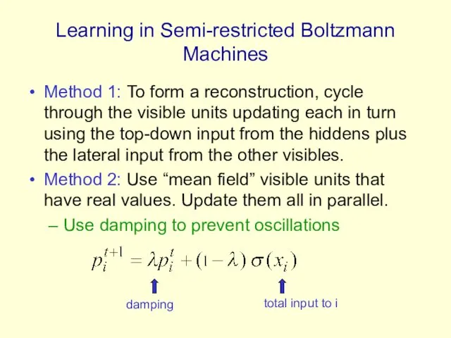
Learning in Semi-restricted Boltzmann Machines
Method 1: To form a reconstruction,
Learning in Semi-restricted Boltzmann Machines
Method 1: To form a reconstruction,
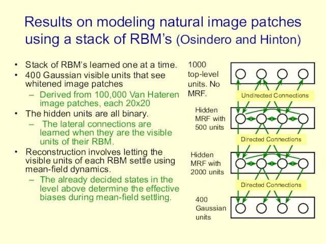
Results on modeling natural image patches using a stack of RBM’s
Results on modeling natural image patches using a stack of RBM’s
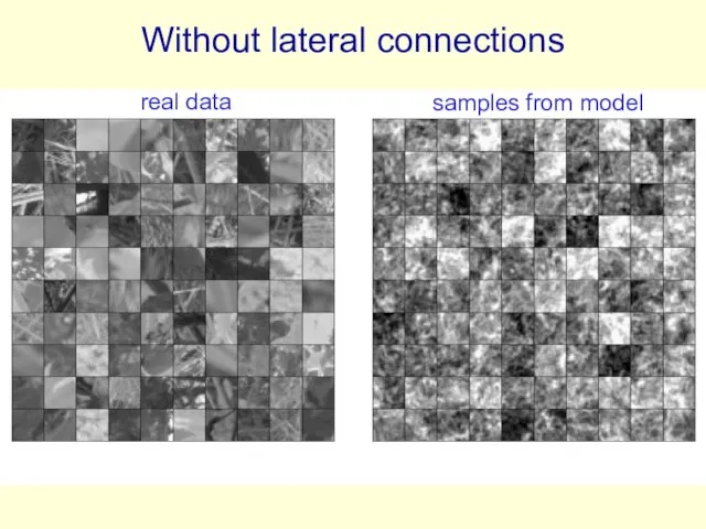
Without lateral connections
real data
samples from model
Without lateral connections
real data
samples from model
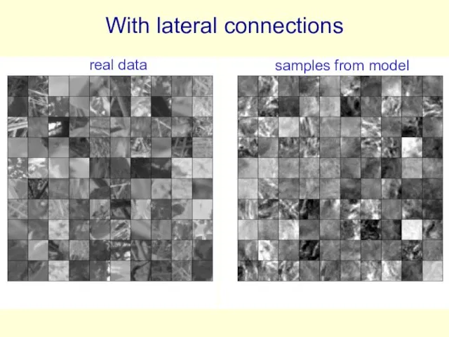
With lateral connections
real data
samples from model
With lateral connections
real data
samples from model
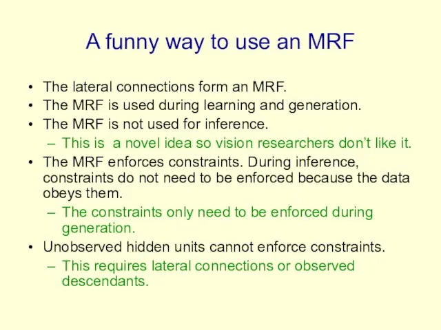
A funny way to use an MRF
The lateral connections form an
A funny way to use an MRF
The lateral connections form an
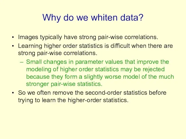
Why do we whiten data?
Images typically have strong pair-wise correlations.
Learning higher
Why do we whiten data?
Images typically have strong pair-wise correlations.
Learning higher
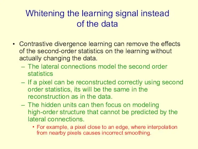
Whitening the learning signal instead of the data
Contrastive divergence learning can
Whitening the learning signal instead of the data
Contrastive divergence learning can
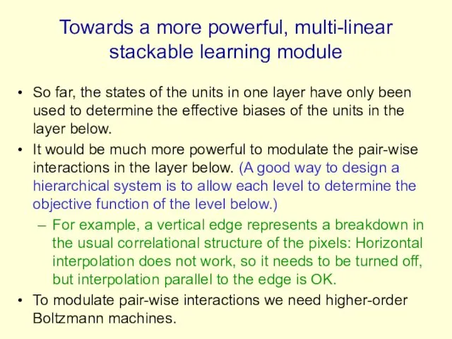
Towards a more powerful, multi-linear stackable learning module
So far, the states
Towards a more powerful, multi-linear stackable learning module
So far, the states
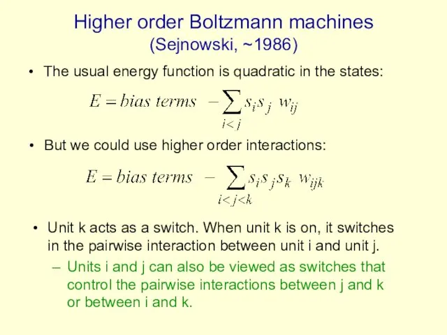
Higher order Boltzmann machines (Sejnowski, ~1986)
The usual energy function is quadratic
Higher order Boltzmann machines (Sejnowski, ~1986)
The usual energy function is quadratic
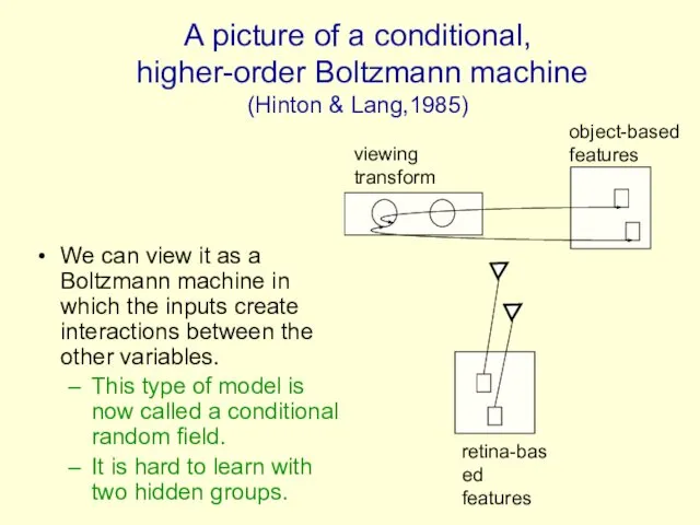
A picture of a conditional,
higher-order Boltzmann machine
(Hinton & Lang,1985)
retina-based
A picture of a conditional,
higher-order Boltzmann machine
(Hinton & Lang,1985)
retina-based
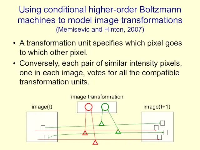
Using conditional higher-order Boltzmann machines to model image transformations (Memisevic and
Using conditional higher-order Boltzmann machines to model image transformations (Memisevic and
 Вспомогательный алгоритм
 Язык разметки гипертекста HTML (Hyper Text Markup Language )
 Использование подзапросов для решения запросов
 Презентация на тему МОДЕЛИРОВАНИЕ И ФОРМАЛИЗАЦИЯ
 Визуализация параметрических исследований
 Смартфон в житті. Застосування в життєвих ситуаціях
 Модели данных в информационных системах
 Файлы и папки
  Правовая информатика
 Компьютерное конструирование. Исходные данные для проектирования модели упорного подшипника скольжения в Компас-3D
 Программалық жабдыққа қатысты талаптармен жұмыс істеу принциптері. Жобалау мәселелері
 Администрирование информационных систем Шифрование
  Create a own Database
 Виртуальный обзор ПК, на который установлено ПО
 Файлы и файловая система
 Презентация по информатике Элементы статистической обработки данных 7 класс
 Представление чисел в памяти компьютера. 10 класс
 Презентация "MSC.Mvision Appendix C" - скачать презентации по Информатике
 Выполнение запросов, создание и редактирование отчета. MS Access
 Графические приемы. Лекция 2
 Тенологія створення кишенькового календаря
 Курс «С#. Программирование на языке высокого уровня» Павловская Т.А.
  Твоя безопасная сеть
 Объектно-ориентированные подходы
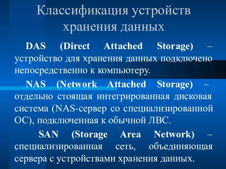 Классификация устройств хранения данных
 Net pay`. Агрегатор электронных платежей
 Министерство образования и науки Республики Башкортостан Государственное бюджетное
 Таблицы HTML - документов