- Geometric Modeling - Parametric Representation of Synthetic Curves

Содержание
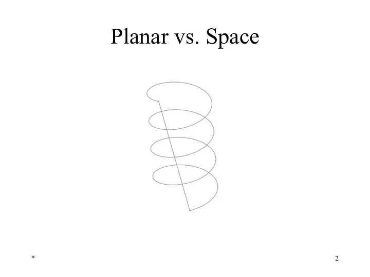
- 2. * Planar vs. Space
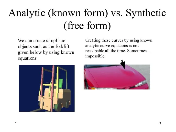
- 3. * Analytic (known form) vs. Synthetic (free form) Creating these curves by using known analytic curve
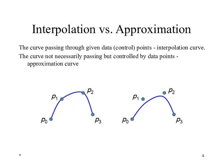
- 4. * Interpolation vs. Approximation The curve passing through given data (control) points - interpolation curve. The
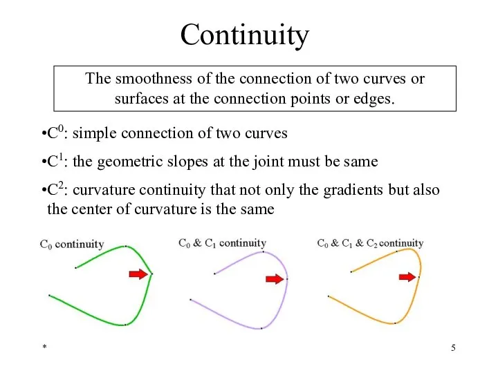
- 5. * Continuity The smoothness of the connection of two curves or surfaces at the connection points
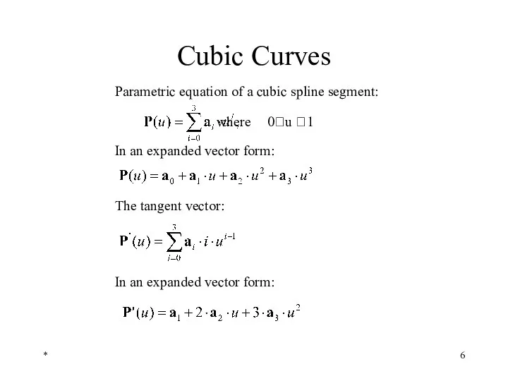
- 6. * Cubic Curves In an expanded vector form: Parametric equation of a cubic spline segment: where
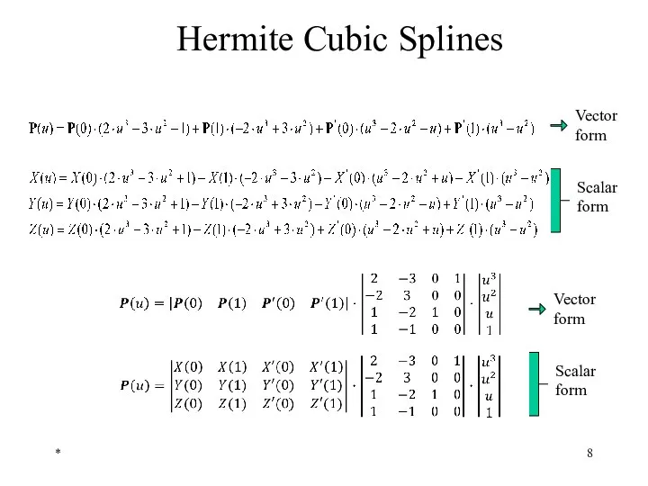
- 7. * Hermite Cubic Splines Hermite form of a general cubic spline is defined by positions and
- 8. * Hermite Cubic Splines
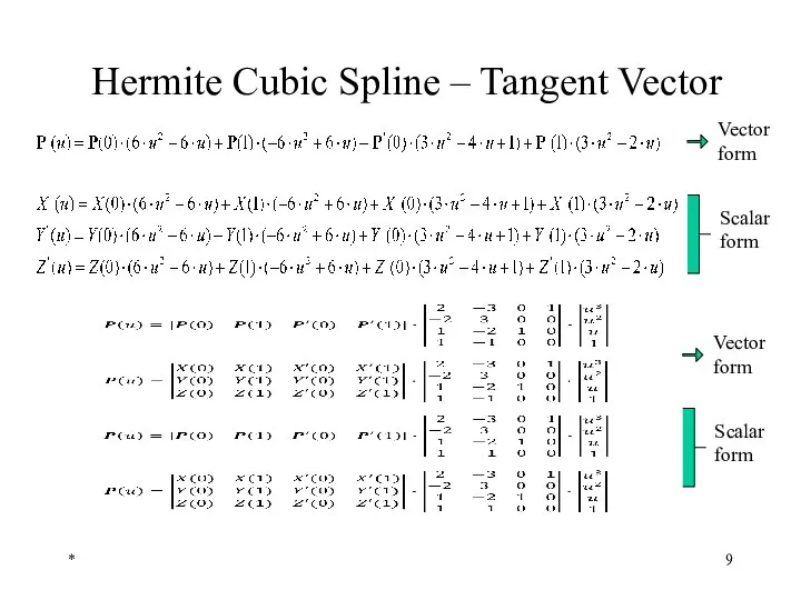
- 9. * Hermite Cubic Spline – Tangent Vector
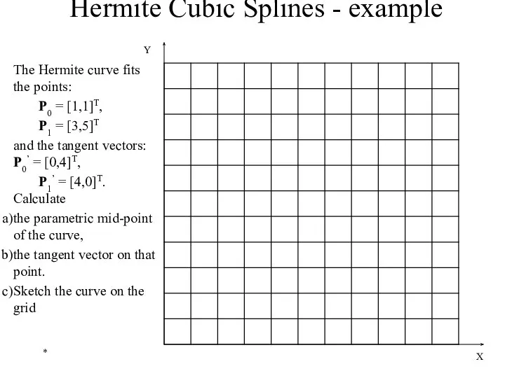
- 10. * X Hermite Cubic Splines - example The Hermite curve fits the points: P0 = [1,1]T,
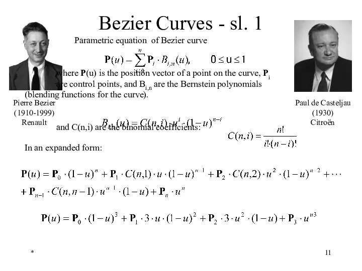
- 11. * Bezier Curves - sl. 1 Parametric equation of Bezier curve where P(u) is the position
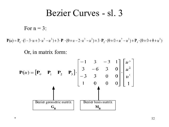
- 12. * Bezier Curves - sl. 3 For n = 3: Bezier basis matrix MB Or, in
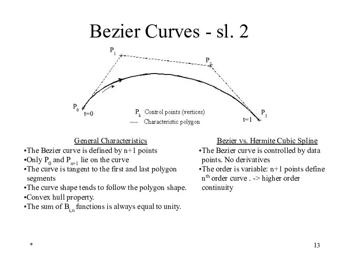
- 13. * Bezier Curves - sl. 2 General Characteristics The Bezier curve is defined by n+1 points
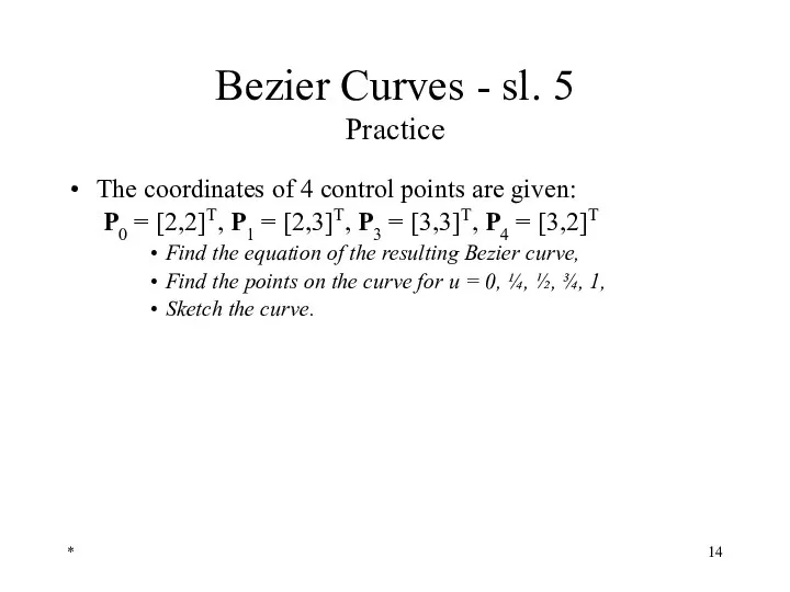
- 14. * Bezier Curves - sl. 5 Practice The coordinates of 4 control points are given: P0
- 15. * Bezier Curves - sl. 4
- 16. * B-spline Curves - sl. 1 See: http://www.ibiblio.org/e-notes/Splines/Basis.htm Powerful generalization of Bezier curves local control opportunity
- 17. * B-spline Curves - sl. 2 See: http://www.ibiblio.org/e-notes/Splines/Basis.htm The B-spline curve defined by n+1 control points
- 18. * B-spline Curves - sl. 3 Basis Functions The function Ni,k determines how strongly control point
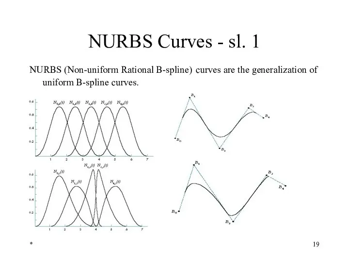
- 19. * NURBS Curves - sl. 1 NURBS (Non-uniform Rational B-spline) curves are the generalization of uniform
- 21. Скачать презентацию
*
Planar vs. Space
*
Planar vs. Space
*
Analytic (known form) vs. Synthetic (free form)
Creating these curves by using
*
Analytic (known form) vs. Synthetic (free form)
Creating these curves by using
*
Interpolation vs. Approximation
The curve passing through given data (control) points
*
Interpolation vs. Approximation
The curve passing through given data (control) points
*
Continuity
The smoothness of the connection of two curves or surfaces at
*
Continuity
The smoothness of the connection of two curves or surfaces at
*
Cubic Curves
In an expanded vector form:
Parametric equation of a cubic spline
*
Cubic Curves
In an expanded vector form:
Parametric equation of a cubic spline

*
Hermite Cubic Splines
Hermite form of a general cubic spline is defined
*
Hermite Cubic Splines
Hermite form of a general cubic spline is defined
*
Hermite Cubic Splines
*
Hermite Cubic Splines
*
Hermite Cubic Spline – Tangent Vector
*
Hermite Cubic Spline – Tangent Vector
*
X
Hermite Cubic Splines - example
The Hermite curve fits the points:
P0
*
X
Hermite Cubic Splines - example
The Hermite curve fits the points:
P0
*
Bezier Curves - sl. 1
Parametric equation of Bezier curve
where P(u)
*
Bezier Curves - sl. 1
Parametric equation of Bezier curve
where P(u)
*
Bezier Curves - sl. 3
For n = 3:
Bezier basis matrix
MB
Or, in
*
Bezier Curves - sl. 3
For n = 3:
Bezier basis matrix
MB
Or, in
*
Bezier Curves - sl. 2
General Characteristics
The Bezier curve is defined by
*
Bezier Curves - sl. 2
General Characteristics
The Bezier curve is defined by
*
Bezier Curves - sl. 5
Practice
The coordinates of 4 control points are
*
Bezier Curves - sl. 5
Practice
The coordinates of 4 control points are
*
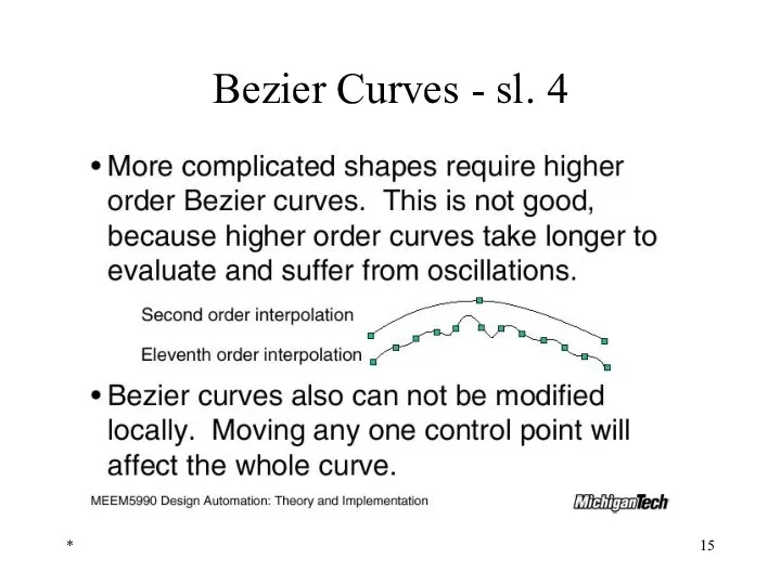
Bezier Curves - sl. 4
*
Bezier Curves - sl. 4
*
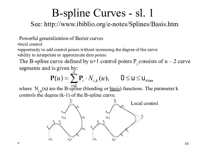
B-spline Curves - sl. 1
See: http://www.ibiblio.org/e-notes/Splines/Basis.htm
Powerful generalization of Bezier curves
local
*
B-spline Curves - sl. 1
See: http://www.ibiblio.org/e-notes/Splines/Basis.htm
Powerful generalization of Bezier curves
local
*
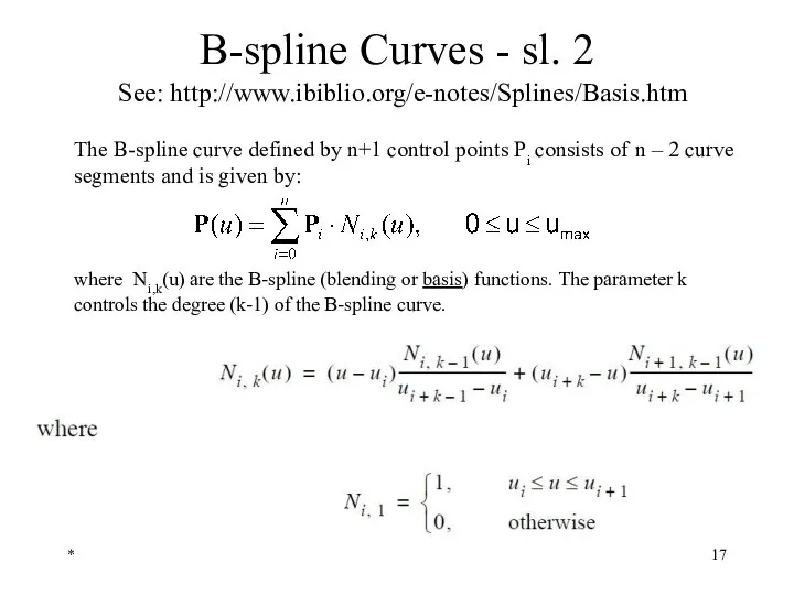
B-spline Curves - sl. 2
See: http://www.ibiblio.org/e-notes/Splines/Basis.htm
The B-spline curve defined by
*
B-spline Curves - sl. 2
See: http://www.ibiblio.org/e-notes/Splines/Basis.htm
The B-spline curve defined by
*
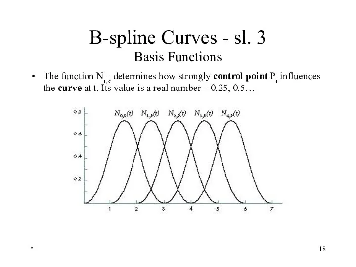
B-spline Curves - sl. 3
Basis Functions
The function Ni,k determines how strongly
*
B-spline Curves - sl. 3
Basis Functions
The function Ni,k determines how strongly
*
NURBS Curves - sl. 1
NURBS (Non-uniform Rational B-spline) curves are the
*
NURBS Curves - sl. 1
NURBS (Non-uniform Rational B-spline) curves are the
 Логика и алгебра высказываний
 Устный счет
  Деление натуральных чисел
 Магия чисел. Нумерология
 Готовимся к ЕГЭ. Задание 23-24
 Степень с рациональным и действительным показателем
 Перпендикуляр и наклонная к прямой
 Обыкновенные дроби и их применение
 Методи вирішення нелінійних рівнянь. (Лекція 3)
 Мы - строители. Обучающая игра-тренажёр. Часть 1
 Вклад мусульманских ученых в развитие геометрии и тригонометрии
 Признаки делимости на 2, 5, 10, 4 и 25. Урок 106
 Применение свойств арифметического квадратного корня
 Справочник по планиметрии. (7-9 класс)
 Сочетательное свойство умножения и сложения
 Решение неравенств ГБОУ СОШ №1084 Учитель математики Смирнова Н.В.
 Состав числа 12
 Определение синуса, косинуса и тангенса угла
 Алгебраические выражения
 Дроби и проценты 6 класс Мовсесова Л.В.
 Нумерология
 Построение графиков функций, содержащих модуль 8 класс Учитель математики МБОУ СОШ № 117 Щербина Антонина Николаевна
  Нахождение дроби от числа
 Презентация по математике "Цель урока – спасти книги" - скачать бесплатно
 Рюкзак. Восстановление ответа
 Проверка статистических гипотез
 Графы и деревья. Кроссворд
 Множественные связи. Порядковые и категоризованные переменные