Environmental Modeling in Industrial Application Models for Supporting Incident Evolution: Release of Dense-than-air Pollutants
- Environmental Modeling in Industrial Application Models for Supporting Incident Evolution: Release of Dense-than-air Pollutants

Содержание
- 2. CONTENTS INTRODUCTION PREVISION MODELS SLAB THEORETICAL DESCRIPTION MODEL ORGANIZATION GOVERNING EQUATIONS TIME AVERAGED CONCENTRATIONS SLAB USER
- 3. INTRODUCTION Emission of polluting substances can come from: Vehicular traffic Industrial plants Thermo-electric plants Natural sources
- 4. INTRODUCTION The spatial and temporal distribution of the concentration of the polluting substance can help to
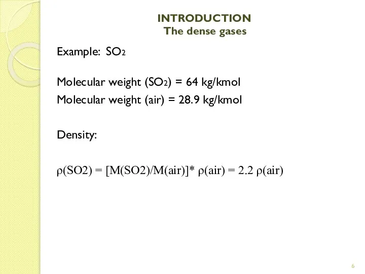
- 5. INTRODUCTION The dense gases The importance of the problem is very high when dealing with: toxic
- 6. INTRODUCTION The dense gases Example: SO2 Molecular weight (SO2) = 64 kg/kmol Molecular weight (air) =
- 7. /24 Airborne chemical pollution Attention must be paid to: accurately determine the types of pollutants taking
- 8. /24 Airborne chemical pollution Pollutants are gaseous mixtures or aerosols, i.e. suspensions of solid or liquid
- 9. /24 Airborne chemical pollution In general, toxic pollutants can penetrate in the organism through: the respiratory
- 10. /24 Airborne chemical pollution An important reference are the tables published and periodically updated by the
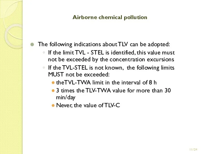
- 11. /24 Airborne chemical pollution The following indications about TLV can be adopted: If the limit TVL
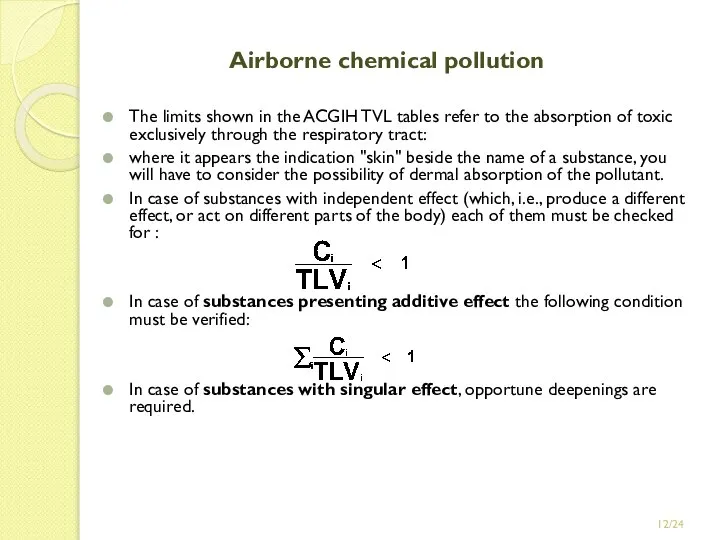
- 12. /24 Airborne chemical pollution The limits shown in the ACGIH TVL tables refer to the absorption
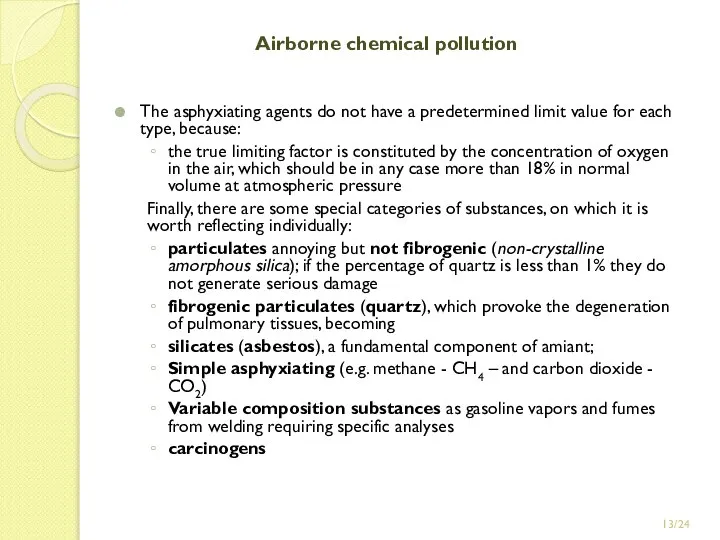
- 13. /24 Airborne chemical pollution The asphyxiating agents do not have a predetermined limit value for each
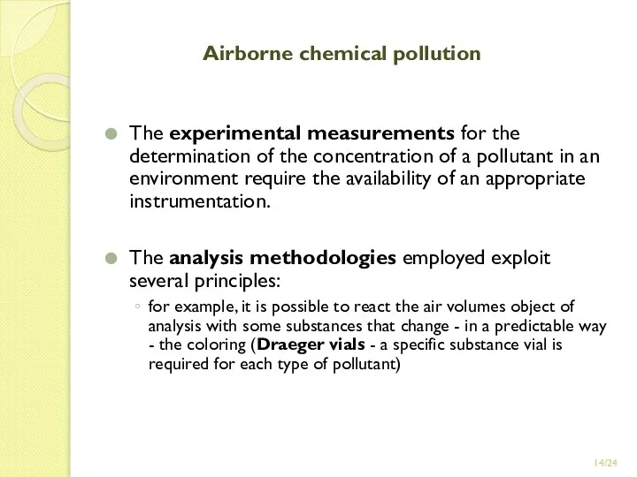
- 14. /24 Airborne chemical pollution The experimental measurements for the determination of the concentration of a pollutant
- 15. /24 Impact on the environment By law, the Chemical Safety Assessment (CSA) and the compiling of
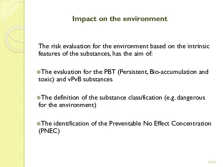
- 16. /24 Impact on the environment The risk evaluation for the environment based on the intrinsic features
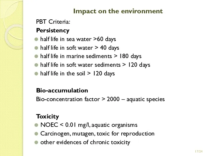
- 17. /24 Impact on the environment PBT Criteria: Persistency half life in sea water >60 days half
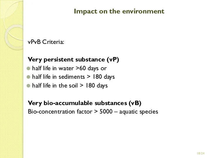
- 18. /24 Impact on the environment vPvB Criteria: Very persistent substance (vP) half life in water >60
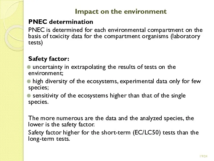
- 19. /24 Impact on the environment PNEC determination PNEC is determined for each environmental compartment on the
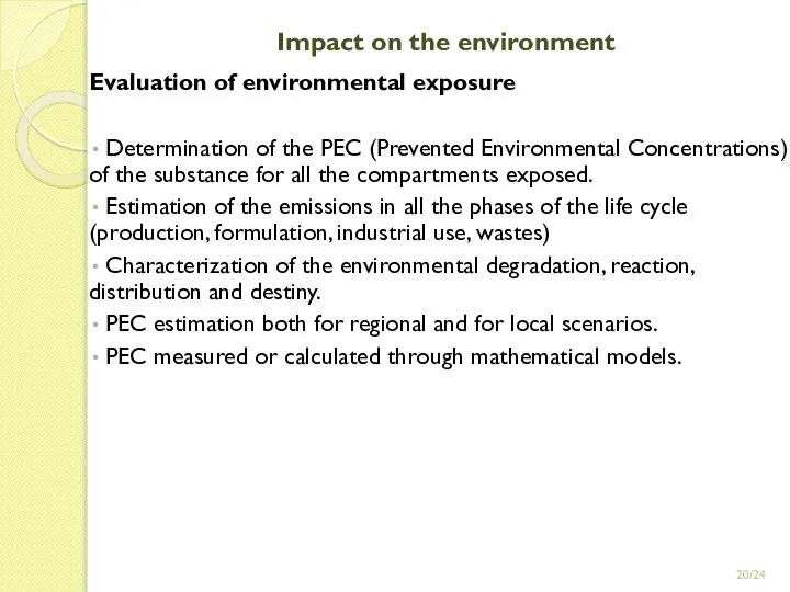
- 20. /24 Impact on the environment Evaluation of environmental exposure Determination of the PEC (Prevented Environmental Concentrations)
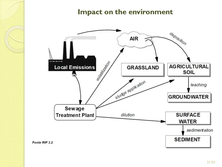
- 21. /24 Impact on the environment
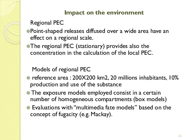
- 22. Impact on the environment Regional PEC Point-shaped releases diffused over a wide area have an effect
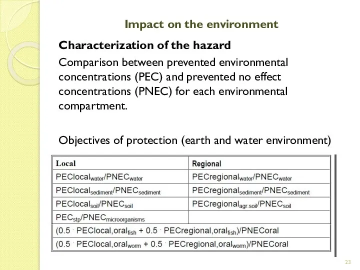
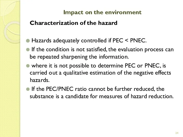
- 23. Impact on the environment Characterization of the hazard Comparison between prevented environmental concentrations (PEC) and prevented
- 24. Impact on the environment Characterization of the hazard Hazards adequately controlled if PEC If the condition
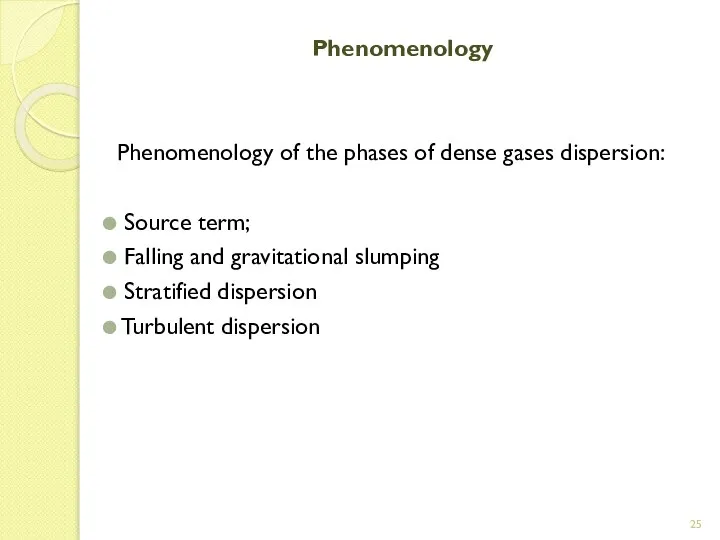
- 25. Phenomenology Phenomenology of the phases of dense gases dispersion: Source term; Falling and gravitational slumping Stratified
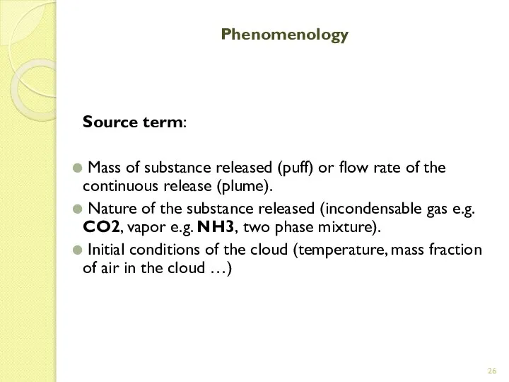
- 26. Phenomenology Source term: Mass of substance released (puff) or flow rate of the continuous release (plume).
- 27. Phenomenology Gravitational slumping of the cloud: The cloud formed by a denser than air release continues
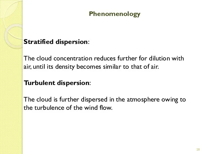
- 28. Phenomenology Stratified dispersion: The cloud concentration reduces further for dilution with air, until its density becomes
- 29. PREVISION MODELS To evaluate and quantify the dispersion of a pollutant emission in the atmosphere, it
- 30. PREVISION MODELS Gaussian models These are very simple analytical codes which require a modest metereologic input
- 31. PREVISION MODELS 3D Lagrangian models They simulate the dispersion of a pollutant through computational particles displaced
- 32. MODELS FOR DENSE GAS RELEASES EVALUATION Open source models DEGADIS SLAB Proprietary models AIRTOX CHARM FOCUS
- 33. MODELS FOR DENSE GAS RELEASES EVALUATION DEGADIS DEGADIS was originally developed for the US Coast Guard
- 34. MODELS FOR DENSE GAS RELEASES EVALUATION SLAB SLAB was developed by Lawrence Livermore National Lab to
- 35. MODELS FOR DENSE GAS RELEASES EVALUATION AIRTOX AIRTOX has been developed by ENSR Consulting and Engineering
- 36. MODELS FOR DENSE GAS RELEASES EVALUATION CHARM CHARM is a Gaussian puff model created by Radian
- 37. MODELS FOR DENSE GAS RELEASES EVALUATION FOCUS FOCUS is a hazards analysis software package designed by
- 38. MODELS FOR DENSE GAS RELEASES EVALUATION SAFEMODE SAFEMODE was developed by Technology and Management Systems Inc.
- 39. MODELS FOR DENSE GAS RELEASES EVALUATION TRACE TRACE was developed by EI Dupont De Nemours Company.
- 40. SLAB
- 41. INTRODUCTION SLAB is a computer code that simulates the atmospheric dispersion of denser than air releases.
- 42. INTRODUCTION Atmospheric dispersion of the release is calculated by solving the conservation equations of Mass Momentum
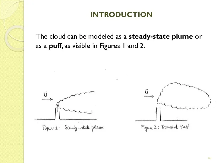
- 43. INTRODUCTION The cloud can be modeled as a steady-state plume or as a puff, as visible
- 44. INTRODUCTION A continuous release (very long emission duration) is treated as a plume. In the case
- 45. INTRODUCTION Solution of the spatially-averaged conservation equations in either dispersion mode yields the spatially-averaged cloud properties.
- 46. INTRODUCTION The time averaged concentration is obtained in a two step process: The effect of the
- 47. MODEL ORGANIZATION Cloud meander effect
- 48. THEORETICAL DESCRIPTION The atmospheric dispersion of a large denser than air release is affected by phenomena
- 49. THEORETICAL DESCRIPTION In combustible gas releases one can be concerned with the instantaneous concentration. In toxic
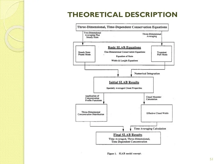
- 50. THEORETICAL DESCRIPTION To meet these requirements, the SLAB model is built upon a theoretical framework that
- 51. THEORETICAL DESCRIPTION
- 52. THEORETICAL DESCRIPTION The conservation equations are different for the two modes, plume and puff. The steady
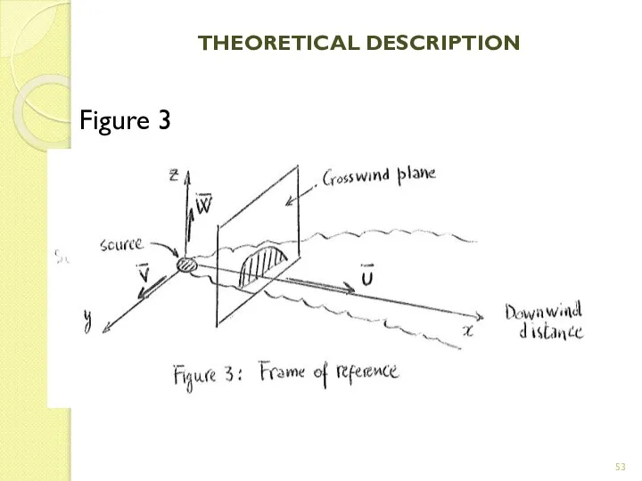
- 53. THEORETICAL DESCRIPTION Figure 3
- 54. THEORETICAL DESCRIPTION The theoretical framework of the SLAB model is completed by the inclusion of the
- 55. THEORETICAL DESCRIPTION To solve the basic set of equations, additional submodels are required. These submodels describe
- 56. THEORETICAL DESCRIPTION The turbulent mixing with surrounding air, is treated by using the entrainment concept which
- 57. THEORETICAL DESCRIPTION In the steady state plume mode the conservation equations are averaged over the cross
- 58. THEORETICAL DESCRIPTION The 3D concentration distribution of the cloud is determined from the average concentration and
- 59. MODEL ORGANIZATION The calculational flow within the SLAB code is reported in Figure below
- 60. MODEL ORGANIZATION There are three stages in a typical simulation: Source identification and initialization for dispersion;
- 61. MODEL ORGANIZATION Dispersion from an evaporating pool and a horizontal jet both begin in the steady
- 62. MODEL ORGANIZATION The situation for the vertical jet is similar to that of the horizontal jet;
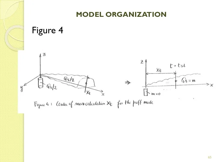
- 63. MODEL ORGANIZATION The dispersion calculation for a continuous but limited release of duration t_sd is initially
- 64. MODEL ORGANIZATION The puff center of mass is set equal to Xt, so that the emitted
- 65. MODEL ORGANIZATION Figure 4
- 66. MODEL ORGANIZATION An exception to this procedure is taken when an evaporating pool release fails to
- 67. MODEL ORGANIZATION Completion of the dispersion calculations in either mode, yields the instantaneous spatially averaged cloud
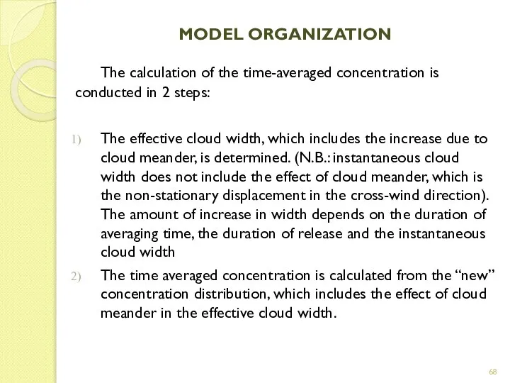
- 68. MODEL ORGANIZATION The calculation of the time-averaged concentration is conducted in 2 steps: The effective cloud
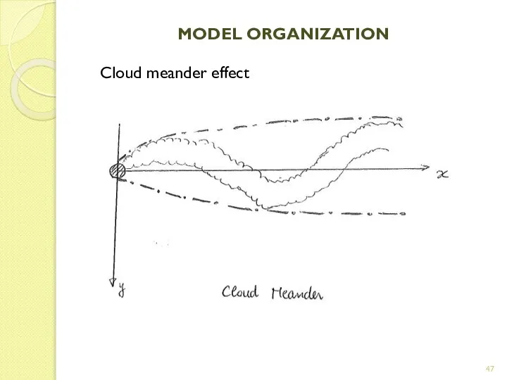
- 69. MODEL ORGANIZATION Cloud meander effect
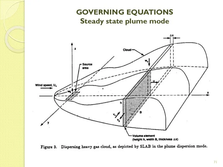
- 70. GOVERNING EQUATIONS Steady state plume mode The steady state plume mode of SLAB is based on
- 71. GOVERNING EQUATIONS Steady state plume mode
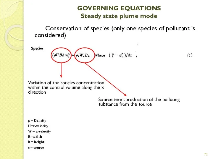
- 72. GOVERNING EQUATIONS Steady state plume mode Conservation of species (only one species of pollutant is considered)
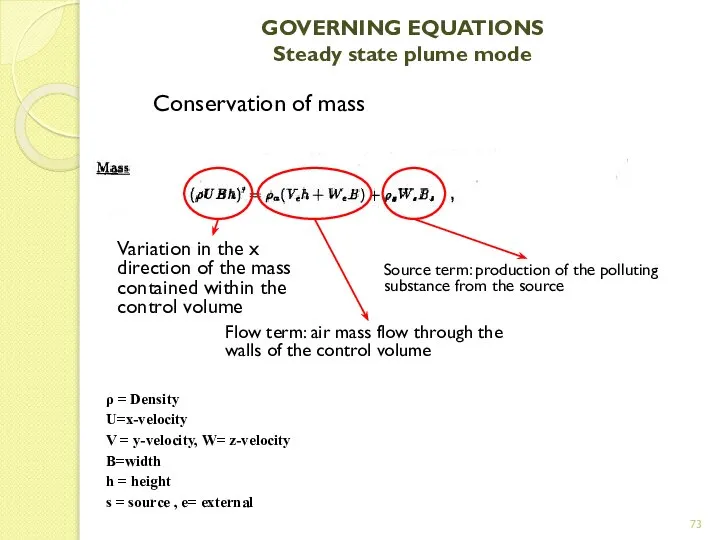
- 73. GOVERNING EQUATIONS Steady state plume mode Conservation of mass Variation in the x direction of the
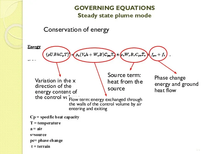
- 74. GOVERNING EQUATIONS Steady state plume mode Conservation of energy Variation in the x direction of the
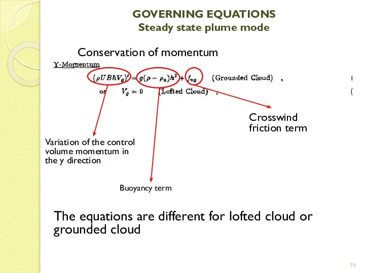
- 75. GOVERNING EQUATIONS Steady state plume mode Conservation of momentum Variation of the control volume momentum in
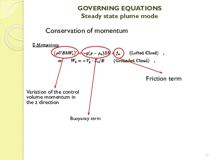
- 76. GOVERNING EQUATIONS Steady state plume mode Conservation of momentum Variation of the control volume momentum in
- 77. GOVERNING EQUATIONS Steady state plume mode Conservation of momentum Variation of the control volume momentum in
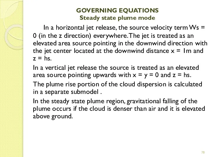
- 78. GOVERNING EQUATIONS Steady state plume mode In a horizontal jet release, the source velocity term Ws
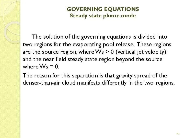
- 79. GOVERNING EQUATIONS Steady state plume mode The solution of the governing equations is divided into two
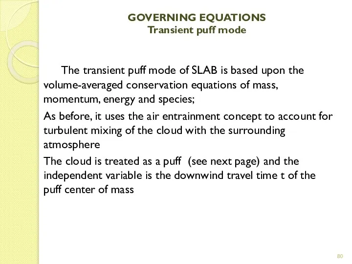
- 80. GOVERNING EQUATIONS Transient puff mode The transient puff mode of SLAB is based upon the volume-averaged
- 81. GOVERNING EQUATIONS Transient puff mode
- 82. GOVERNING EQUATIONS Transient puff mode
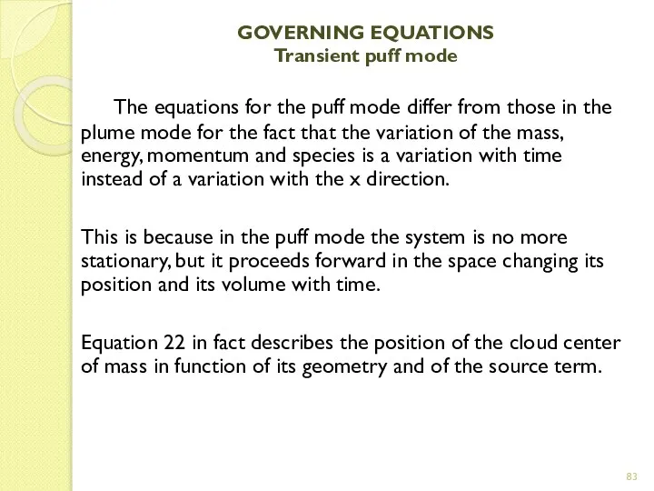
- 83. GOVERNING EQUATIONS Transient puff mode The equations for the puff mode differ from those in the
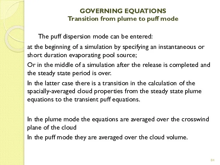
- 84. GOVERNING EQUATIONS Transition from plume to puff mode The puff dispersion mode can be entered: at
- 85. GOVERNING EQUATIONS Transition from plume to puff mode To begin the puff mode calculation it is
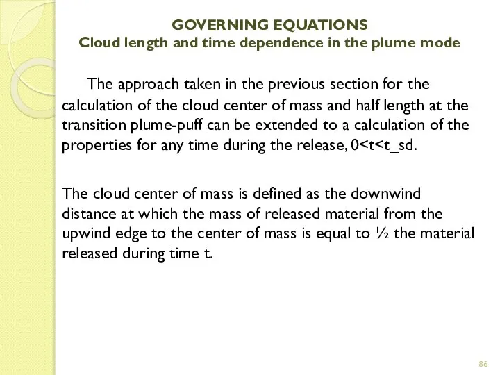
- 86. GOVERNING EQUATIONS Cloud length and time dependence in the plume mode The approach taken in the
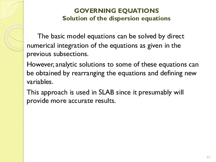
- 87. GOVERNING EQUATIONS Solution of the dispersion equations The basic model equations can be solved by direct
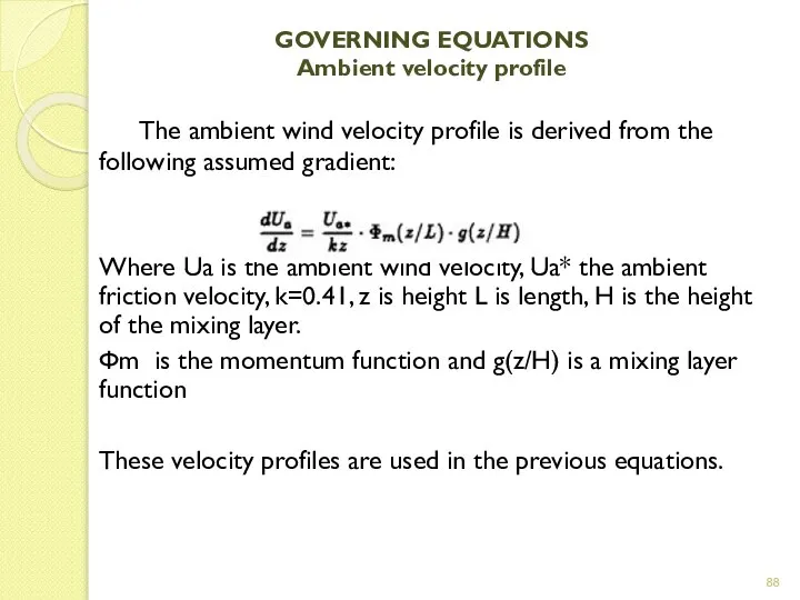
- 88. GOVERNING EQUATIONS Ambient velocity profile The ambient wind velocity profile is derived from the following assumed
- 89. GOVERNING EQUATIONS Entrainment rates The vertical entrainment rate includes the effects of surface friction, differential motion
- 90. GOVERNING EQUATIONS Heat and momentum flux terms The flux terms are adapted from Zeman (1982). The
- 91. GOVERNING EQUATIONS Thermodynamic model Liquid droplets formation and evaporation is governed by an equilibrium thermodynamic model
- 92. GOVERNING EQUATIONS Plume rise The plume from a vertical jet or stack release initially rises until
- 93. TIME AVERAGED CONCENTRATIONS All of the SLAB results (concentration, cloud width …) represent ensemble averages. An
- 94. TIME AVERAGED CONCENTRATIONS
- 95. TIME AVERAGED CONCENTRATIONS in addition to the ensemble average, SLAB uses two other average types: Spatial
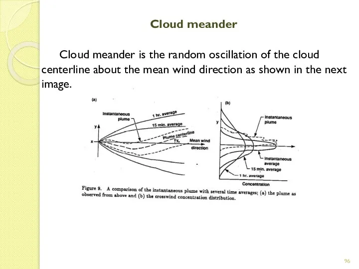
- 96. Cloud meander Cloud meander is the random oscillation of the cloud centerline about the mean wind
- 97. Cloud meander When the cloud concentration os averaged over time, the effective width of the cloud
- 98. Cloud meander In SLAB code solution to the dispersion equations, the cloud meander is ignored and
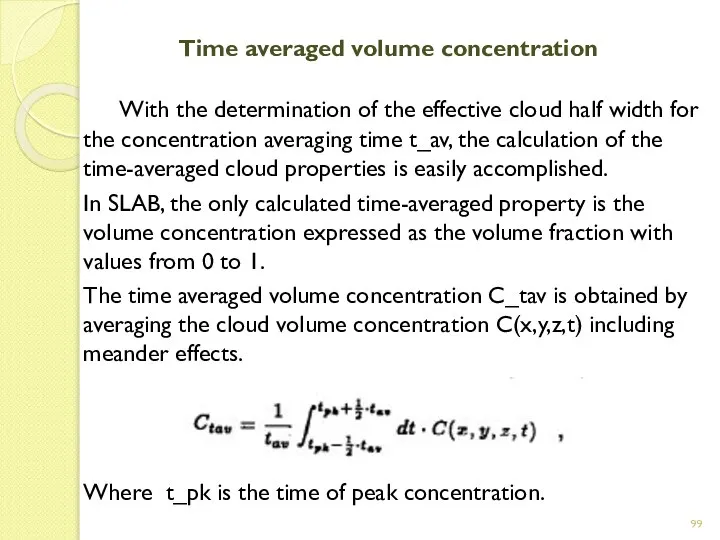
- 99. Time averaged volume concentration With the determination of the effective cloud half width for the concentration
- 100. SLAB User’s guide
- 101. General information SLAB is implemented in the Fortran 77 language. SLAB operates by acquiring an input
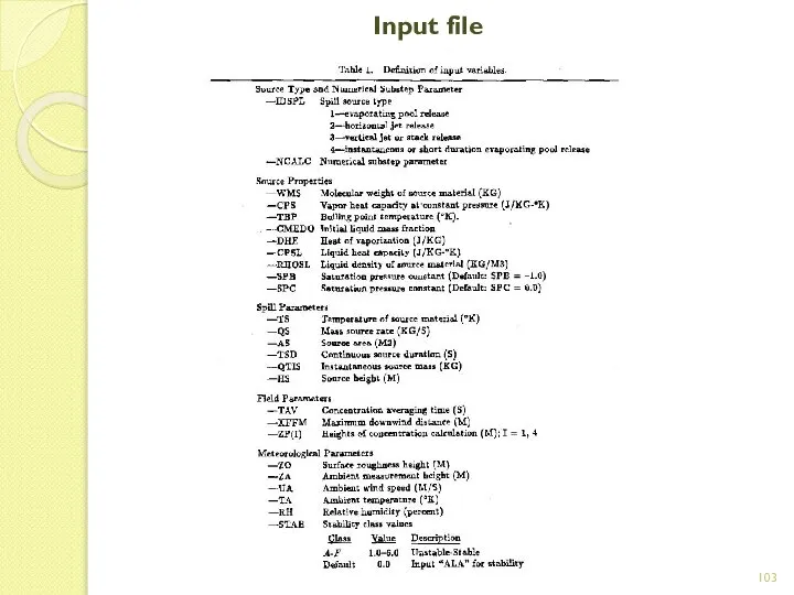
- 102. Input file There are 30 possible input parameters required to run in SLAB. Such parameters include
- 103. Input file
- 104. Source type and numerical substep parameter IDSPL – Spill source type SLAB has 4 types of
- 105. Source type and numerical substep parameter Figure 5
- 106. Source type and numerical substep parameter The evaporating pool is a ground level area source of
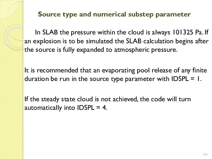
- 107. Source type and numerical substep parameter The vertical jet release is an area source with source
- 108. Source type and numerical substep parameter In SLAB the pressure within the cloud is always 101325
- 109. Source type and numerical substep parameter The parameter NCALC is an integer substep multiplier that specifies
- 110. Source properties WMS = molecular weight of the source material [kg] CPS = vapor heat capacity
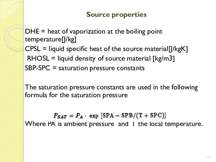
- 111. Source properties DHE = heat of vaporization at the boiling point temperature[J/kg] CPSL = liquid specific
- 112. Source properties Some examples of substances are here provided
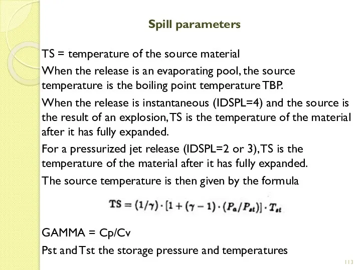
- 113. Spill parameters TS = temperature of the source material When the release is an evaporating pool,
- 114. Spill parameters QS = mass source rate [kg/s]4 For an instantaneous release, the QS value should
- 115. Spill parameters TSD = continuous source duration [s] This parameter specifies the duration of the release
- 116. Field parameters TAV = concentration averaging time [s] The concentration averaging time is the appropriate averaging
- 117. Field parameters XFFM=maximum downwind distance [m] This is the maximum downwind (x) distance for which the
- 118. Meteo parameters ZO = surface roughness height [m] Is generally estimated in two ways: The first
- 119. Meteo parameters ZA = ambient measurement height [m] This is the height at which ambient windspeed
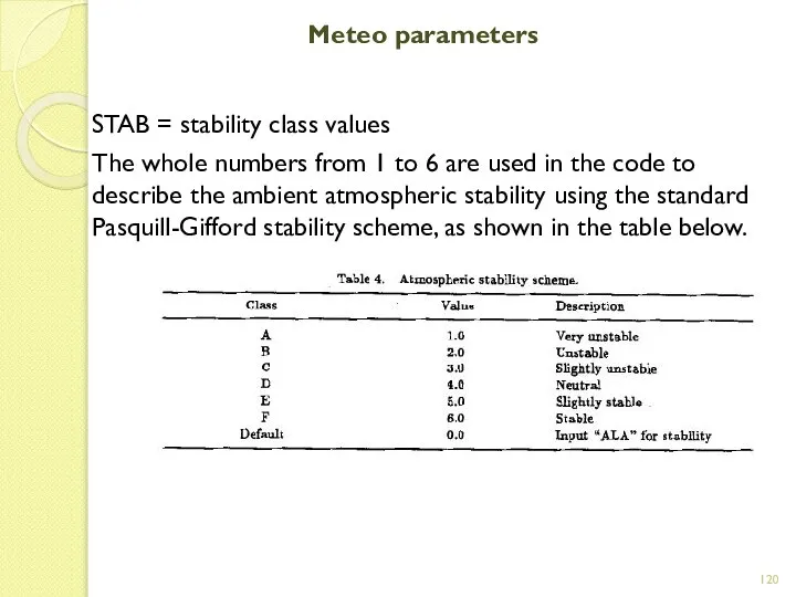
- 120. Meteo parameters STAB = stability class values The whole numbers from 1 to 6 are used
- 121. Meteo parameters The classes of atmospheric stability are an method of classification of the atmospheric stability,
- 122. Meteo parameters ALA = inverse Monin-Obukhov length [1/m] This is a stability parameter used to describe
- 123. Meteo parameters The Obukhov length is used to describe the effects of buoyancy on turbulent flows,
- 124. Input file closure After the code has read the input and executed a run, it returns
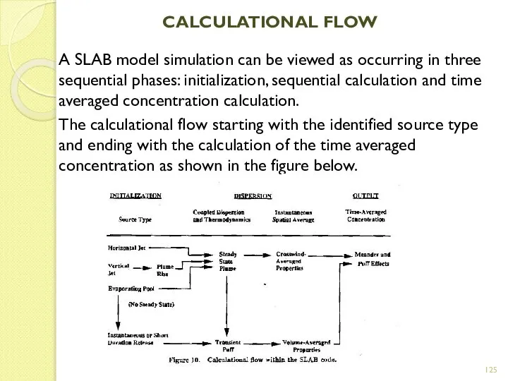
- 125. CALCULATIONAL FLOW A SLAB model simulation can be viewed as occurring in three sequential phases: initialization,
- 126. CALCULATIONAL FLOW Initialization The initialization begins with the specification of the source type. There is one
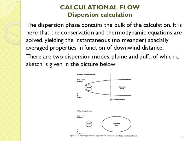
- 127. CALCULATIONAL FLOW Dispersion calculation The dispersion phase contains the bulk of the calculation. It is here
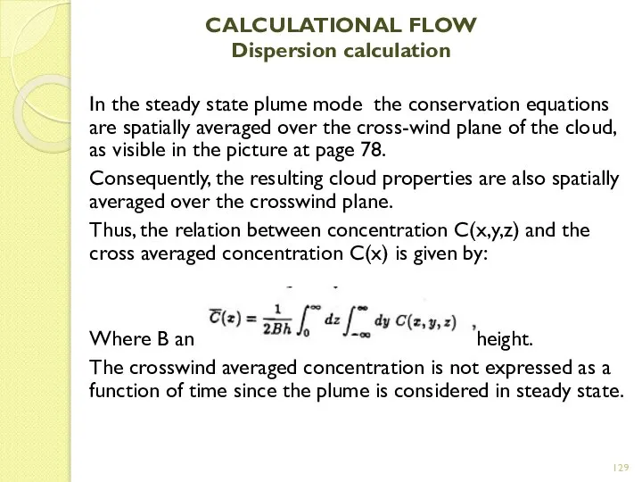
- 128. CALCULATIONAL FLOW Dispersion calculation The steady state plume mode is used for the finite duration releases
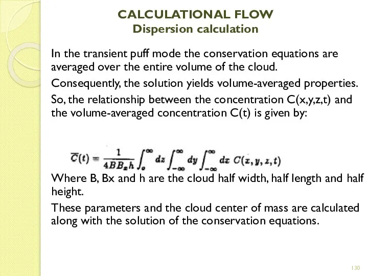
- 129. CALCULATIONAL FLOW Dispersion calculation In the steady state plume mode the conservation equations are spatially averaged
- 130. CALCULATIONAL FLOW Dispersion calculation In the transient puff mode the conservation equations are averaged over the
- 131. CALCULATIONAL FLOW Dispersion calculation In the transient puff mode the conservation equations are averaged over the
- 132. CALCULATIONAL FLOW Time averaged concentration calculation After the spatially-averaged cloud properties are calculated at all downwind
- 133. CALCULATIONAL FLOW Time averaged concentration calculation The calculation of the time averaged volume fraction C_tav(x,y,z,t) from
- 134. CALCULATIONAL FLOW Time averaged concentration calculation The time available for cloud meander at the downwind location
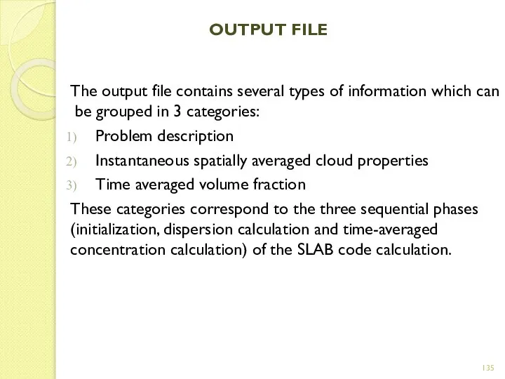
- 135. OUTPUT FILE The output file contains several types of information which can be grouped in 3
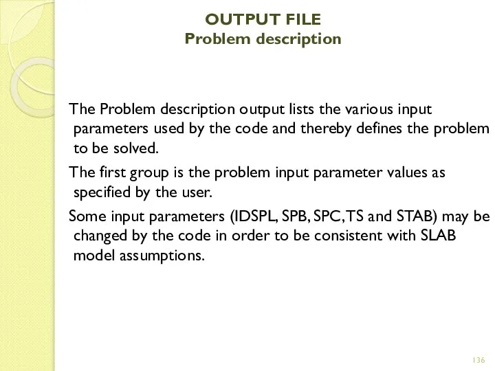
- 136. OUTPUT FILE Problem description The Problem description output lists the various input parameters used by the
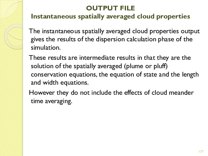
- 137. OUTPUT FILE Instantaneous spatially averaged cloud properties The instantaneous spatially averaged cloud properties output gives the
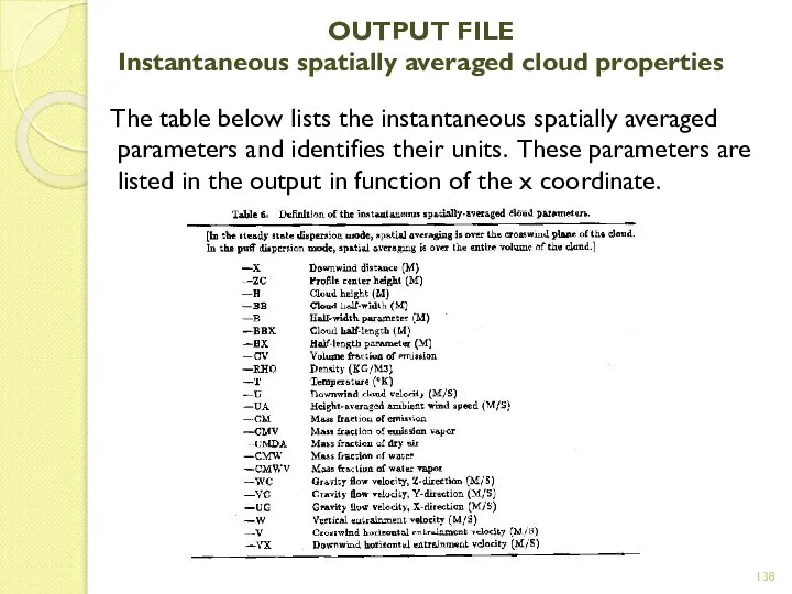
- 138. OUTPUT FILE Instantaneous spatially averaged cloud properties The table below lists the instantaneous spatially averaged parameters
- 139. OUTPUT FILE Instantaneous spatially averaged cloud properties The cloud properties listed before, are described as “instantaneous”
- 140. OUTPUT FILE Instantaneous spatially averaged cloud properties The “spatial” averaging in SLAB is of 2 types:
- 141. OUTPUT FILE Time averaged volume fraction In SLAB the time averaged concentration is expressed as the
- 142. OUTPUT FILE Time averaged volume fraction The concentration contour parameters output lists a number of parameters
- 143. OUTPUT FILE Time averaged volume fraction The concentration in the Z=ZP(I) plane gives the the time
- 144. OUTPUT FILE Time averaged volume fraction The final result is the maximum centerline concentration. Here the
- 146. Скачать презентацию
CONTENTS
INTRODUCTION
PREVISION MODELS
SLAB
THEORETICAL DESCRIPTION
MODEL ORGANIZATION
GOVERNING EQUATIONS
TIME AVERAGED CONCENTRATIONS
SLAB USER GUIDE
CONTENTS
INTRODUCTION
PREVISION MODELS
SLAB
THEORETICAL DESCRIPTION
MODEL ORGANIZATION
GOVERNING EQUATIONS
TIME AVERAGED CONCENTRATIONS
SLAB USER GUIDE
INTRODUCTION
Emission of polluting substances can come from:
Vehicular traffic
Industrial plants
Thermo-electric plants
Natural
INTRODUCTION
Emission of polluting substances can come from:
Vehicular traffic
Industrial plants
Thermo-electric plants
Natural
INTRODUCTION
The spatial and temporal distribution of the concentration of the polluting
INTRODUCTION
The spatial and temporal distribution of the concentration of the polluting

INTRODUCTION
The dense gases
The importance of the problem is very high when
INTRODUCTION
The dense gases
The importance of the problem is very high when
INTRODUCTION
The dense gases
Example: SO2
Molecular weight (SO2) = 64 kg/kmol
Molecular weight
INTRODUCTION
The dense gases
Example: SO2
Molecular weight (SO2) = 64 kg/kmol
Molecular weight
/24
Airborne chemical pollution
Attention must be paid to:
accurately determine the types of
/24
Airborne chemical pollution
Attention must be paid to:
accurately determine the types of
/24
Airborne chemical pollution
Pollutants are gaseous mixtures or aerosols, i.e. suspensions of
/24
Airborne chemical pollution
Pollutants are gaseous mixtures or aerosols, i.e. suspensions of
/24
Airborne chemical pollution
In general, toxic pollutants can penetrate in the organism
/24
Airborne chemical pollution
In general, toxic pollutants can penetrate in the organism
/24
Airborne chemical pollution
An important reference are the tables published and periodically
/24
Airborne chemical pollution
An important reference are the tables published and periodically
/24
Airborne chemical pollution
The following indications about TLV can be adopted:
If the
/24
Airborne chemical pollution
The following indications about TLV can be adopted:
If the
/24
Airborne chemical pollution
The limits shown in the ACGIH TVL tables refer
/24
Airborne chemical pollution
The limits shown in the ACGIH TVL tables refer
/24
Airborne chemical pollution
The asphyxiating agents do not have a predetermined limit
/24
Airborne chemical pollution
The asphyxiating agents do not have a predetermined limit
/24
Airborne chemical pollution
The experimental measurements for the determination of the concentration
/24
Airborne chemical pollution
The experimental measurements for the determination of the concentration

/24
Impact on the environment
By law, the Chemical Safety Assessment (CSA) and
/24
Impact on the environment
By law, the Chemical Safety Assessment (CSA) and
/24
Impact on the environment
The risk evaluation for the environment based on
/24
Impact on the environment
The risk evaluation for the environment based on
/24
Impact on the environment
PBT Criteria:
Persistency
half life in sea
/24
Impact on the environment
PBT Criteria:
Persistency
half life in sea
/24
Impact on the environment
vPvB Criteria:
Very persistent substance (vP)
half life
/24
Impact on the environment
vPvB Criteria:
Very persistent substance (vP)
half life
/24
Impact on the environment
PNEC determination
PNEC is determined for each environmental compartment
/24
Impact on the environment
PNEC determination
PNEC is determined for each environmental compartment
/24
Impact on the environment
Evaluation of environmental exposure
Determination of the PEC
/24
Impact on the environment
Evaluation of environmental exposure
Determination of the PEC
/24
Impact on the environment
/24
Impact on the environment
Impact on the environment
Regional PEC
Point-shaped releases diffused over a wide area
Impact on the environment
Regional PEC
Point-shaped releases diffused over a wide area
Impact on the environment
Characterization of the hazard
Comparison between prevented environmental concentrations
Impact on the environment
Characterization of the hazard
Comparison between prevented environmental concentrations
Impact on the environment
Characterization of the hazard
Hazards adequately controlled if
Impact on the environment
Characterization of the hazard
Hazards adequately controlled if
Phenomenology
Phenomenology of the phases of dense gases dispersion:
Source term;
Falling
Phenomenology
Phenomenology of the phases of dense gases dispersion:
Source term;
Falling
Phenomenology
Source term:
Mass of substance released (puff) or flow rate of
Phenomenology
Source term:
Mass of substance released (puff) or flow rate of

Phenomenology
Gravitational slumping of the cloud:
The cloud formed by a denser than
Phenomenology
Gravitational slumping of the cloud:
The cloud formed by a denser than
Phenomenology
Stratified dispersion:
The cloud concentration reduces further for dilution with air, until
Phenomenology
Stratified dispersion:
The cloud concentration reduces further for dilution with air, until
PREVISION MODELS
To evaluate and quantify the dispersion of a pollutant emission
PREVISION MODELS
To evaluate and quantify the dispersion of a pollutant emission
PREVISION MODELS
Gaussian models
These are very simple analytical codes which require a
PREVISION MODELS
Gaussian models
These are very simple analytical codes which require a
PREVISION MODELS
3D Lagrangian models
They simulate the dispersion of a pollutant through
PREVISION MODELS
3D Lagrangian models
They simulate the dispersion of a pollutant through
MODELS FOR DENSE GAS RELEASES EVALUATION
Open source models
DEGADIS
SLAB
Proprietary models
AIRTOX
CHARM
FOCUS
SAFEMODE
TRACE
MODELS FOR DENSE GAS RELEASES EVALUATION
Open source models
DEGADIS
SLAB
Proprietary models
AIRTOX
CHARM
FOCUS
SAFEMODE
TRACE
MODELS FOR DENSE GAS RELEASES EVALUATION
DEGADIS
DEGADIS was originally developed for the
MODELS FOR DENSE GAS RELEASES EVALUATION
DEGADIS
DEGADIS was originally developed for the

MODELS FOR DENSE GAS RELEASES EVALUATION
SLAB
SLAB was developed by Lawrence Livermore
MODELS FOR DENSE GAS RELEASES EVALUATION
SLAB
SLAB was developed by Lawrence Livermore
MODELS FOR DENSE GAS RELEASES EVALUATION
AIRTOX
AIRTOX has been developed by ENSR
MODELS FOR DENSE GAS RELEASES EVALUATION
AIRTOX
AIRTOX has been developed by ENSR
MODELS FOR DENSE GAS RELEASES EVALUATION
CHARM
CHARM is a Gaussian puff model
MODELS FOR DENSE GAS RELEASES EVALUATION
CHARM
CHARM is a Gaussian puff model
MODELS FOR DENSE GAS RELEASES EVALUATION
FOCUS
FOCUS is a hazards analysis software
MODELS FOR DENSE GAS RELEASES EVALUATION
FOCUS
FOCUS is a hazards analysis software

MODELS FOR DENSE GAS RELEASES EVALUATION
SAFEMODE
SAFEMODE was developed by Technology and
MODELS FOR DENSE GAS RELEASES EVALUATION
SAFEMODE
SAFEMODE was developed by Technology and
MODELS FOR DENSE GAS RELEASES EVALUATION
TRACE
TRACE was developed by EI Dupont
MODELS FOR DENSE GAS RELEASES EVALUATION
TRACE
TRACE was developed by EI Dupont

SLAB
SLAB
INTRODUCTION
SLAB is a computer code that simulates the atmospheric dispersion of
INTRODUCTION
SLAB is a computer code that simulates the atmospheric dispersion of
INTRODUCTION
Atmospheric dispersion of the release is calculated by solving the conservation
INTRODUCTION
Atmospheric dispersion of the release is calculated by solving the conservation
INTRODUCTION
The cloud can be modeled as a steady-state plume or as
INTRODUCTION
The cloud can be modeled as a steady-state plume or as
INTRODUCTION
A continuous release (very long emission duration) is treated as a
INTRODUCTION
A continuous release (very long emission duration) is treated as a

INTRODUCTION
Solution of the spatially-averaged conservation equations in either dispersion mode yields
INTRODUCTION
Solution of the spatially-averaged conservation equations in either dispersion mode yields
INTRODUCTION
The time averaged concentration is obtained in a two step process:
INTRODUCTION
The time averaged concentration is obtained in a two step process:
MODEL ORGANIZATION
Cloud meander effect
MODEL ORGANIZATION
Cloud meander effect
THEORETICAL DESCRIPTION
The atmospheric dispersion of a large denser than air release
THEORETICAL DESCRIPTION
The atmospheric dispersion of a large denser than air release
THEORETICAL DESCRIPTION
In combustible gas releases one can be concerned with the
THEORETICAL DESCRIPTION
In combustible gas releases one can be concerned with the
THEORETICAL DESCRIPTION
To meet these requirements, the SLAB model is built upon
THEORETICAL DESCRIPTION
To meet these requirements, the SLAB model is built upon
THEORETICAL DESCRIPTION
THEORETICAL DESCRIPTION

THEORETICAL DESCRIPTION
The conservation equations are different for the two modes, plume
THEORETICAL DESCRIPTION
The conservation equations are different for the two modes, plume
THEORETICAL DESCRIPTION
Figure 3
THEORETICAL DESCRIPTION
Figure 3
THEORETICAL DESCRIPTION
The theoretical framework of the SLAB model is completed by
THEORETICAL DESCRIPTION
The theoretical framework of the SLAB model is completed by
THEORETICAL DESCRIPTION
To solve the basic set of equations, additional submodels are
THEORETICAL DESCRIPTION
To solve the basic set of equations, additional submodels are
THEORETICAL DESCRIPTION
The turbulent mixing with surrounding air, is treated by using
THEORETICAL DESCRIPTION
The turbulent mixing with surrounding air, is treated by using
THEORETICAL DESCRIPTION
In the steady state plume mode the conservation equations are
THEORETICAL DESCRIPTION
In the steady state plume mode the conservation equations are
THEORETICAL DESCRIPTION
The 3D concentration distribution of the cloud is determined from
THEORETICAL DESCRIPTION
The 3D concentration distribution of the cloud is determined from

MODEL ORGANIZATION
The calculational flow within the SLAB code is reported in
MODEL ORGANIZATION
The calculational flow within the SLAB code is reported in
MODEL ORGANIZATION
There are three stages in a typical simulation:
Source identification
MODEL ORGANIZATION
There are three stages in a typical simulation:
Source identification

MODEL ORGANIZATION
Dispersion from an evaporating pool and a horizontal jet both
MODEL ORGANIZATION
Dispersion from an evaporating pool and a horizontal jet both
MODEL ORGANIZATION
The situation for the vertical jet is similar to that
MODEL ORGANIZATION
The situation for the vertical jet is similar to that
MODEL ORGANIZATION
The dispersion calculation for a continuous but limited release of
MODEL ORGANIZATION
The dispersion calculation for a continuous but limited release of

MODEL ORGANIZATION
The puff center of mass is set equal to Xt,
MODEL ORGANIZATION
The puff center of mass is set equal to Xt,
MODEL ORGANIZATION
Figure 4
MODEL ORGANIZATION
Figure 4

MODEL ORGANIZATION
An exception to this procedure is taken when an evaporating
MODEL ORGANIZATION
An exception to this procedure is taken when an evaporating

MODEL ORGANIZATION
Completion of the dispersion calculations in either mode, yields the
MODEL ORGANIZATION
Completion of the dispersion calculations in either mode, yields the
MODEL ORGANIZATION
The calculation of the time-averaged concentration is conducted in 2
MODEL ORGANIZATION
The calculation of the time-averaged concentration is conducted in 2

MODEL ORGANIZATION
Cloud meander effect
MODEL ORGANIZATION
Cloud meander effect

GOVERNING EQUATIONS
Steady state plume mode
The steady state plume mode of SLAB
GOVERNING EQUATIONS
Steady state plume mode
The steady state plume mode of SLAB
GOVERNING EQUATIONS
Steady state plume mode
GOVERNING EQUATIONS
Steady state plume mode
GOVERNING EQUATIONS
Steady state plume mode
Conservation of species (only one species of
GOVERNING EQUATIONS
Steady state plume mode
Conservation of species (only one species of
GOVERNING EQUATIONS
Steady state plume mode
Conservation of mass
Variation in the x direction
GOVERNING EQUATIONS
Steady state plume mode
Conservation of mass
Variation in the x direction
GOVERNING EQUATIONS
Steady state plume mode
Conservation of energy
Variation in the x direction
GOVERNING EQUATIONS
Steady state plume mode
Conservation of energy
Variation in the x direction

GOVERNING EQUATIONS
Steady state plume mode
Conservation of momentum
Variation of the control volume
GOVERNING EQUATIONS
Steady state plume mode
Conservation of momentum
Variation of the control volume
GOVERNING EQUATIONS
Steady state plume mode
Conservation of momentum
Variation of the control volume
GOVERNING EQUATIONS
Steady state plume mode
Conservation of momentum
Variation of the control volume
GOVERNING EQUATIONS
Steady state plume mode
Conservation of momentum
Variation of the control volume
GOVERNING EQUATIONS
Steady state plume mode
Conservation of momentum
Variation of the control volume
GOVERNING EQUATIONS
Steady state plume mode
In a horizontal jet release, the source
GOVERNING EQUATIONS
Steady state plume mode
In a horizontal jet release, the source
GOVERNING EQUATIONS
Steady state plume mode
The solution of the governing equations is
GOVERNING EQUATIONS
Steady state plume mode
The solution of the governing equations is
GOVERNING EQUATIONS
Transient puff mode
The transient puff mode of SLAB is based
GOVERNING EQUATIONS
Transient puff mode
The transient puff mode of SLAB is based

GOVERNING EQUATIONS
Transient puff mode
GOVERNING EQUATIONS
Transient puff mode

GOVERNING EQUATIONS
Transient puff mode
GOVERNING EQUATIONS
Transient puff mode
GOVERNING EQUATIONS
Transient puff mode
The equations for the puff mode differ from
GOVERNING EQUATIONS
Transient puff mode
The equations for the puff mode differ from
GOVERNING EQUATIONS
Transition from plume to puff mode
The puff dispersion mode can
GOVERNING EQUATIONS
Transition from plume to puff mode
The puff dispersion mode can

GOVERNING EQUATIONS
Transition from plume to puff mode
To begin the puff mode
GOVERNING EQUATIONS
Transition from plume to puff mode
To begin the puff mode
GOVERNING EQUATIONS
Cloud length and time dependence in the plume mode
The approach
GOVERNING EQUATIONS
Cloud length and time dependence in the plume mode
The approach
GOVERNING EQUATIONS
Solution of the dispersion equations
The basic model equations can be
GOVERNING EQUATIONS
Solution of the dispersion equations
The basic model equations can be
GOVERNING EQUATIONS
Ambient velocity profile
The ambient wind velocity profile is derived from
GOVERNING EQUATIONS
Ambient velocity profile
The ambient wind velocity profile is derived from
GOVERNING EQUATIONS
Entrainment rates
The vertical entrainment rate includes the effects of surface
GOVERNING EQUATIONS
Entrainment rates
The vertical entrainment rate includes the effects of surface

GOVERNING EQUATIONS
Heat and momentum flux terms
The flux terms are adapted from
GOVERNING EQUATIONS
Heat and momentum flux terms
The flux terms are adapted from
GOVERNING EQUATIONS
Thermodynamic model
Liquid droplets formation and evaporation is governed by an
GOVERNING EQUATIONS
Thermodynamic model
Liquid droplets formation and evaporation is governed by an

GOVERNING EQUATIONS
Plume rise
The plume from a vertical jet or stack release
GOVERNING EQUATIONS
Plume rise
The plume from a vertical jet or stack release
TIME AVERAGED CONCENTRATIONS
All of the SLAB results (concentration, cloud width …)
TIME AVERAGED CONCENTRATIONS
All of the SLAB results (concentration, cloud width …)

TIME AVERAGED CONCENTRATIONS
TIME AVERAGED CONCENTRATIONS
TIME AVERAGED CONCENTRATIONS
in addition to the ensemble average, SLAB uses two
TIME AVERAGED CONCENTRATIONS
in addition to the ensemble average, SLAB uses two
Cloud meander
Cloud meander is the random oscillation of the cloud centerline
Cloud meander
Cloud meander is the random oscillation of the cloud centerline

Cloud meander
When the cloud concentration os averaged over time, the effective
Cloud meander
When the cloud concentration os averaged over time, the effective
Cloud meander
In SLAB code solution to the dispersion equations, the cloud
Cloud meander
In SLAB code solution to the dispersion equations, the cloud
Time averaged volume concentration
With the determination of the effective cloud half
Time averaged volume concentration
With the determination of the effective cloud half
SLAB
User’s guide
SLAB
User’s guide
General information
SLAB is implemented in the Fortran 77 language.
SLAB operates by
General information
SLAB is implemented in the Fortran 77 language.
SLAB operates by

Input file
There are 30 possible input parameters required to run in
Input file
There are 30 possible input parameters required to run in
Input file
Input file
Source type and numerical substep parameter
IDSPL – Spill source type
SLAB has
Source type and numerical substep parameter
IDSPL – Spill source type
SLAB has
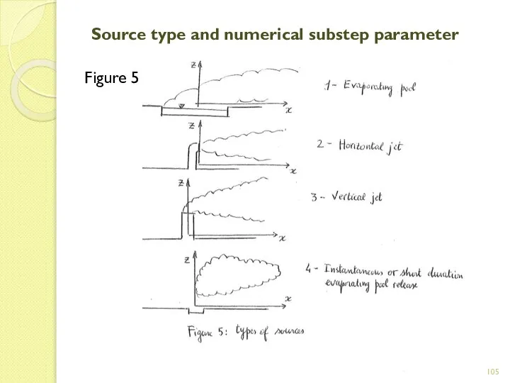
Source type and numerical substep parameter
Figure 5
Source type and numerical substep parameter
Figure 5

Source type and numerical substep parameter
The evaporating pool is a ground
Source type and numerical substep parameter
The evaporating pool is a ground

Source type and numerical substep parameter
The vertical jet release is an
Source type and numerical substep parameter
The vertical jet release is an
Source type and numerical substep parameter
In SLAB the pressure within the
Source type and numerical substep parameter
In SLAB the pressure within the
Source type and numerical substep parameter
The parameter NCALC is an integer
Source type and numerical substep parameter
The parameter NCALC is an integer
![Source properties WMS = molecular weight of the source material [kg]](/_ipx/f_webp&q_80&fit_contain&s_1440x1080/imagesDir/jpg/1410478/slide-109.jpg)
Source properties
WMS = molecular weight of the source material [kg]
CPS =
Source properties
WMS = molecular weight of the source material [kg]
CPS =
Source properties
DHE = heat of vaporization at the boiling point temperature[J/kg]
CPSL
Source properties
DHE = heat of vaporization at the boiling point temperature[J/kg]
CPSL

Source properties
Some examples of substances are here provided
Source properties
Some examples of substances are here provided
Spill parameters
TS = temperature of the source material
When the release
Spill parameters
TS = temperature of the source material
When the release
![Spill parameters QS = mass source rate [kg/s]4 For an instantaneous](/_ipx/f_webp&q_80&fit_contain&s_1440x1080/imagesDir/jpg/1410478/slide-113.jpg)
Spill parameters
QS = mass source rate [kg/s]4
For an instantaneous release, the
Spill parameters
QS = mass source rate [kg/s]4
For an instantaneous release, the
![Spill parameters TSD = continuous source duration [s] This parameter specifies](/_ipx/f_webp&q_80&fit_contain&s_1440x1080/imagesDir/jpg/1410478/slide-114.jpg)
Spill parameters
TSD = continuous source duration [s]
This parameter specifies the duration
Spill parameters
TSD = continuous source duration [s]
This parameter specifies the duration
![Field parameters TAV = concentration averaging time [s] The concentration averaging](/_ipx/f_webp&q_80&fit_contain&s_1440x1080/imagesDir/jpg/1410478/slide-115.jpg)
Field parameters
TAV = concentration averaging time [s]
The concentration averaging time is
Field parameters
TAV = concentration averaging time [s]
The concentration averaging time is
![Field parameters XFFM=maximum downwind distance [m] This is the maximum downwind](/_ipx/f_webp&q_80&fit_contain&s_1440x1080/imagesDir/jpg/1410478/slide-116.jpg)
Field parameters
XFFM=maximum downwind distance [m]
This is the maximum downwind (x) distance
Field parameters
XFFM=maximum downwind distance [m]
This is the maximum downwind (x) distance
![Meteo parameters ZO = surface roughness height [m] Is generally estimated](/_ipx/f_webp&q_80&fit_contain&s_1440x1080/imagesDir/jpg/1410478/slide-117.jpg)
Meteo parameters
ZO = surface roughness height [m]
Is generally estimated in two
Meteo parameters
ZO = surface roughness height [m]
Is generally estimated in two
![Meteo parameters ZA = ambient measurement height [m] This is the](/_ipx/f_webp&q_80&fit_contain&s_1440x1080/imagesDir/jpg/1410478/slide-118.jpg)
Meteo parameters
ZA = ambient measurement height [m]
This is the height at
Meteo parameters
ZA = ambient measurement height [m]
This is the height at
Meteo parameters
STAB = stability class values
The whole numbers from 1 to
Meteo parameters
STAB = stability class values
The whole numbers from 1 to
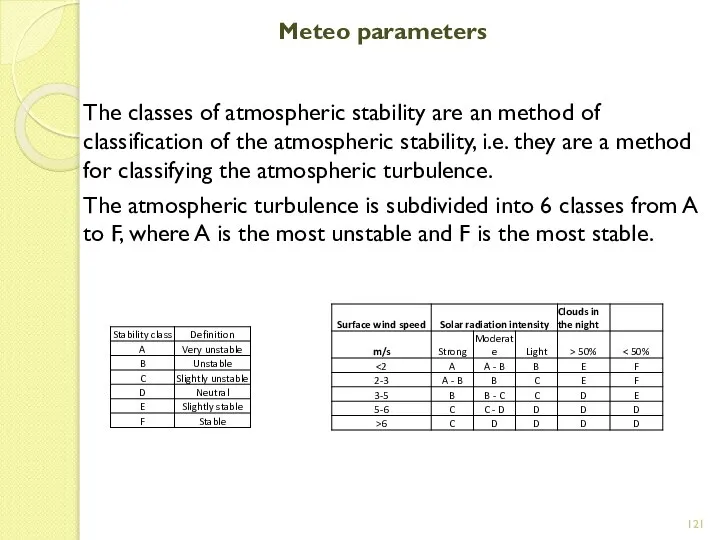
Meteo parameters
The classes of atmospheric stability are an method of classification
Meteo parameters
The classes of atmospheric stability are an method of classification
![Meteo parameters ALA = inverse Monin-Obukhov length [1/m] This is a](/_ipx/f_webp&q_80&fit_contain&s_1440x1080/imagesDir/jpg/1410478/slide-121.jpg)
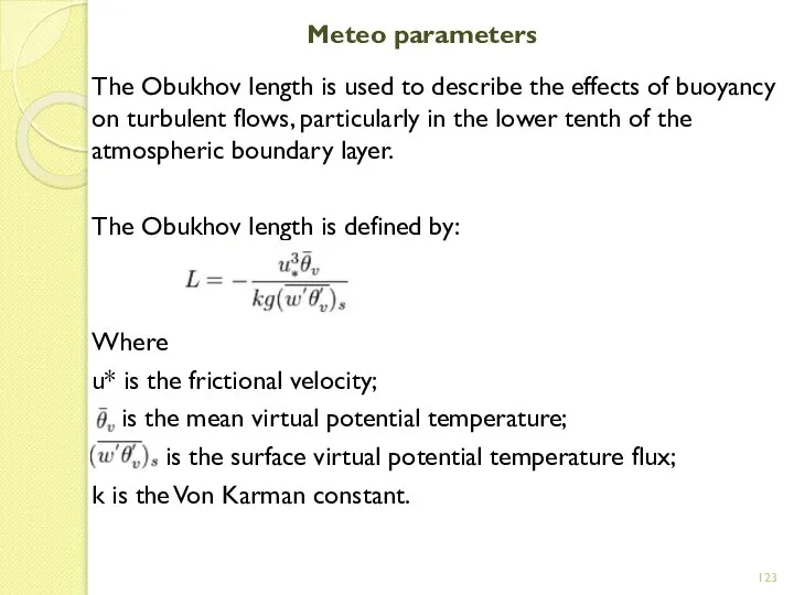
Meteo parameters
ALA = inverse Monin-Obukhov length [1/m]
This is a stability parameter
Meteo parameters
ALA = inverse Monin-Obukhov length [1/m]
This is a stability parameter
Meteo parameters
The Obukhov length is used to describe the effects of
Meteo parameters
The Obukhov length is used to describe the effects of
Input file closure
After the code has read the input and executed
Input file closure
After the code has read the input and executed
CALCULATIONAL FLOW
A SLAB model simulation can be viewed as occurring in
CALCULATIONAL FLOW
A SLAB model simulation can be viewed as occurring in

CALCULATIONAL FLOW
Initialization
The initialization begins with the specification of the source type.
There
CALCULATIONAL FLOW
Initialization
The initialization begins with the specification of the source type.
There
CALCULATIONAL FLOW
Dispersion calculation
The dispersion phase contains the bulk of the calculation.
CALCULATIONAL FLOW
Dispersion calculation
The dispersion phase contains the bulk of the calculation.
CALCULATIONAL FLOW
Dispersion calculation
The steady state plume mode is used for the
CALCULATIONAL FLOW
Dispersion calculation
The steady state plume mode is used for the
CALCULATIONAL FLOW
Dispersion calculation
In the steady state plume mode the conservation equations
CALCULATIONAL FLOW
Dispersion calculation
In the steady state plume mode the conservation equations
CALCULATIONAL FLOW
Dispersion calculation
In the transient puff mode the conservation equations are
CALCULATIONAL FLOW
Dispersion calculation
In the transient puff mode the conservation equations are

CALCULATIONAL FLOW
Dispersion calculation
In the transient puff mode the conservation equations are
CALCULATIONAL FLOW
Dispersion calculation
In the transient puff mode the conservation equations are
CALCULATIONAL FLOW
Time averaged concentration calculation
After the spatially-averaged cloud properties are calculated
CALCULATIONAL FLOW
Time averaged concentration calculation
After the spatially-averaged cloud properties are calculated
CALCULATIONAL FLOW
Time averaged concentration calculation
The calculation of the time averaged volume
CALCULATIONAL FLOW
Time averaged concentration calculation
The calculation of the time averaged volume
CALCULATIONAL FLOW
Time averaged concentration calculation
The time available for cloud meander at
CALCULATIONAL FLOW
Time averaged concentration calculation
The time available for cloud meander at
OUTPUT FILE
The output file contains several types of information which can
OUTPUT FILE
The output file contains several types of information which can
OUTPUT FILE
Problem description
The Problem description output lists the various input parameters
OUTPUT FILE
Problem description
The Problem description output lists the various input parameters
OUTPUT FILE
Instantaneous spatially averaged cloud properties
The instantaneous spatially averaged cloud properties
OUTPUT FILE
Instantaneous spatially averaged cloud properties
The instantaneous spatially averaged cloud properties
OUTPUT FILE
Instantaneous spatially averaged cloud properties
The table below lists the instantaneous
OUTPUT FILE
Instantaneous spatially averaged cloud properties
The table below lists the instantaneous
OUTPUT FILE
Instantaneous spatially averaged cloud properties
The cloud properties listed before, are
OUTPUT FILE
Instantaneous spatially averaged cloud properties
The cloud properties listed before, are
OUTPUT FILE
Instantaneous spatially averaged cloud properties
The “spatial” averaging in SLAB is
OUTPUT FILE
Instantaneous spatially averaged cloud properties
The “spatial” averaging in SLAB is
OUTPUT FILE
Time averaged volume fraction
In SLAB the time averaged concentration is
OUTPUT FILE
Time averaged volume fraction
In SLAB the time averaged concentration is
OUTPUT FILE
Time averaged volume fraction
The concentration contour parameters output lists a
OUTPUT FILE
Time averaged volume fraction
The concentration contour parameters output lists a
OUTPUT FILE
Time averaged volume fraction
The concentration in the Z=ZP(I) plane gives
OUTPUT FILE
Time averaged volume fraction
The concentration in the Z=ZP(I) plane gives
OUTPUT FILE
Time averaged volume fraction
The final result is the maximum centerline
OUTPUT FILE
Time averaged volume fraction
The final result is the maximum centerline
 Сохранение природы средней полосы России от вторжения борщевика Сосновского
 Живоносный Родник - старейший целебный источник города Пензы
 Экосистемный подход к окружающей среде
 Охрана природы
 Химико-экологические проблемы и охрана атмосферы, стратосферы, гидросферы и литосферы
 Ақтөбе қаласының қоныстану аумақтарының атмосфералық ауасының ластануы есебінен канцерогендік емес қауіптілік әсерлерін бағала
 Биологические основы земледелия
 Цепи питания. Поток энергии
 Химическое загрязнение биосферы и здоровье человека
 Класифікація екосистем . Ландшафтна,провінційна і субстратна екосистеми
 Презентация Путешествие колобка
  Природоохранные экологические организации
 Қоғам мен табиғаттың әрекеттесу стратегиясы. Қ.Р. тұрақты дамуға өтудегі концепциясы
 Проблемы охраны гидросферы
 Развитие лесного хозяйства РФ на 2013-2020 годы
 Экология сообществ и экосистем
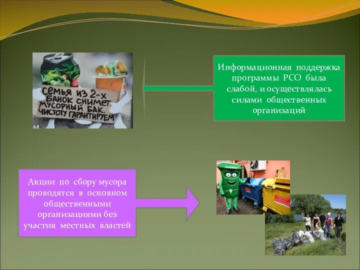 Акции по сбору мусора
 Червона книга України (3 клас)
 Экологические факторы
 Критерии оценки качества окружающей среды
 From smog into jewels
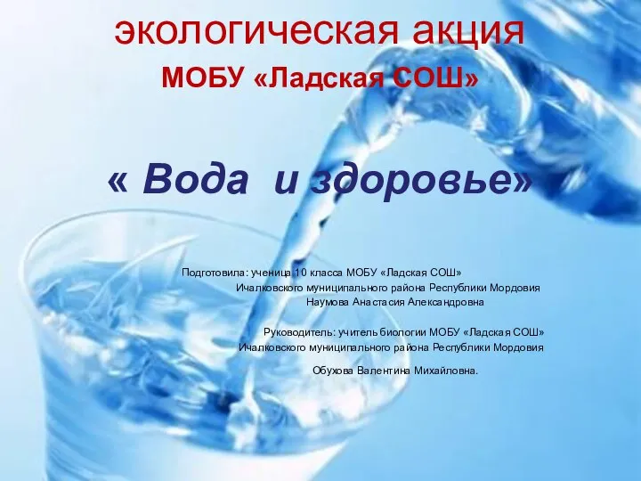 Экологическая акция МОБУ «Ладская СОШ» «Вода и здоровье»
 Понятие экологического аудита
 Экологические проблемы животных
 Потребность человечества в дыхании и ее влияние на биосферу
 Аттестационная работа. Разработка по выполнению исследовательского проекта на уроках биологии и экологии. (8-9 класс)
 Классификация животных. Основные систематические группы. Влияние человека на животных
 Реалии раздельного сбора отходов производства и потребления в структурных подразделениях СКЖД – филиала ОАО «РЖД»