- Scheduling and lot sizing

Содержание
- 2. JAP Scheduling means the allocation of resources over time to accomplish specific tasks. Workforce scheduling determines
- 3. JAP The two basic manufacturing environments are: A JOB SHOP (Process focused system) is a process
- 4. JAP Single Processor Scheduling (no alternative routing) In some cases an entire plant can be viewed
- 5. JAP Allocate your customers to ABC-classes A class –strategic customers / most profitable (or other vice
- 6. JAP Typically scheduling is divided to: Rough planning - > Master Production Schedule MPS (months and
- 7. JAP Rough planning – MPS What are the main objectives, reasoning and steps of it?
- 8. JAP TASK 1: Estimating realistic delivery times Specially needed for sales – for customer promises
- 9. JAP TASK 2: Ensuring the resources needed Specially needed to keep the delivery time promises given
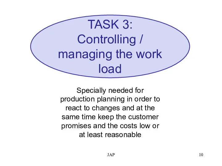
- 10. JAP TASK 3: Controlling / managing the work load Specially needed for production planning in order
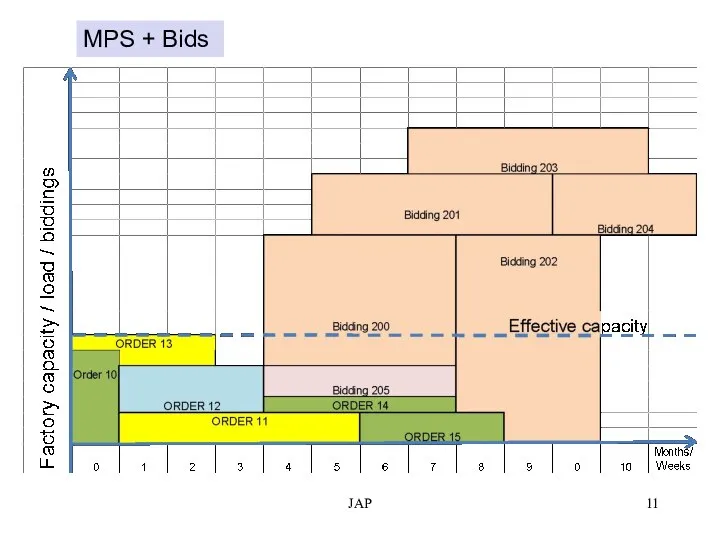
- 11. JAP MPS + Bids
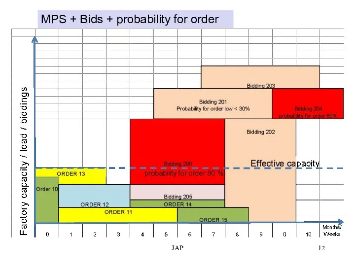
- 12. JAP MPS + Bids + probability for order
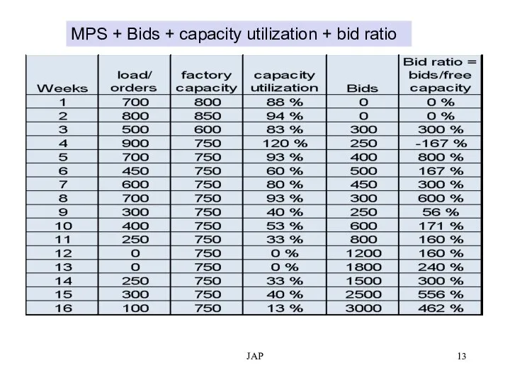
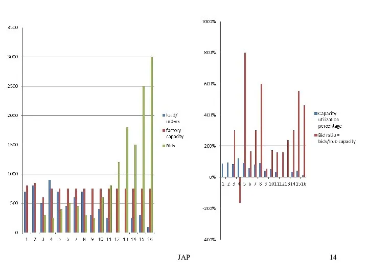
- 13. JAP MPS + Bids + capacity utilization + bid ratio
- 14. JAP
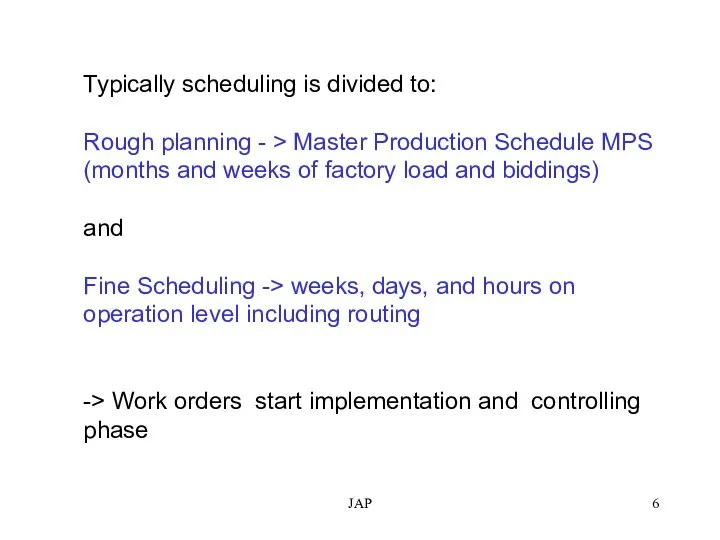
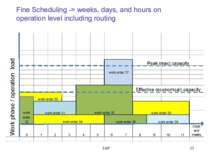
- 15. JAP Fine Scheduling -> weeks, days, and hours on operation level including routing
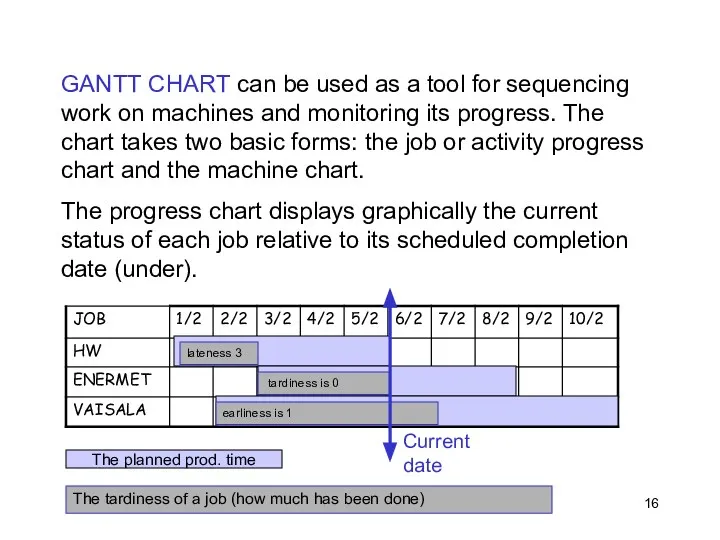
- 16. JAP GANTT CHART can be used as a tool for sequencing work on machines and monitoring
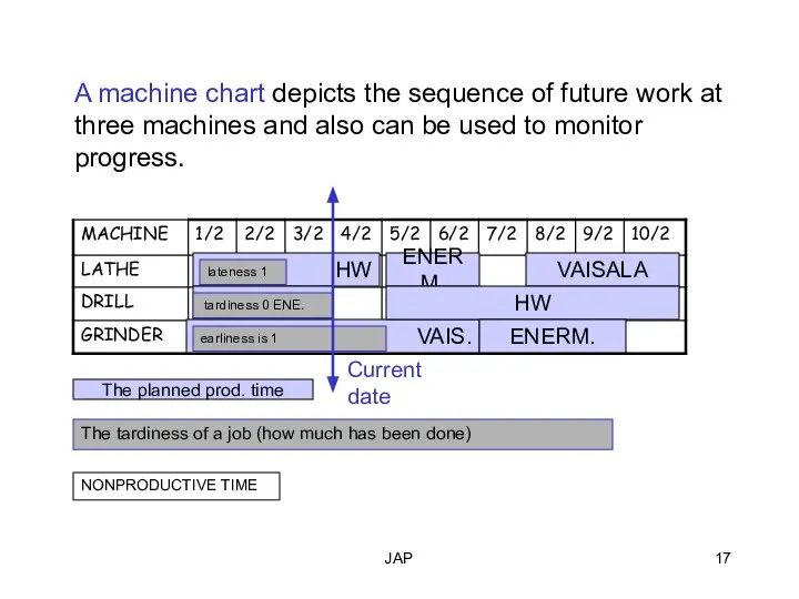
- 17. JAP A machine chart depicts the sequence of future work at three machines and also can
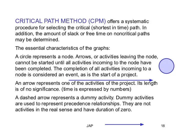
- 18. JAP CRITICAL PATH METHOD (CPM) offers a systematic procedure for selecting the critical (shortest in time)
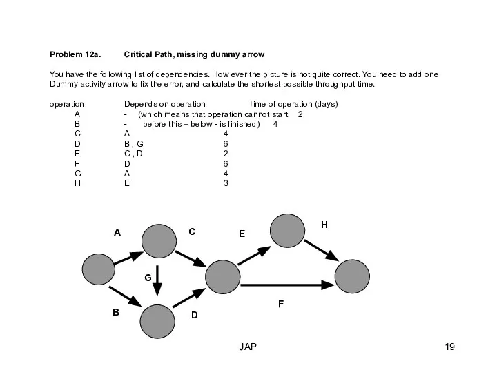
- 19. G A B E F H C D Problem 12a. Critical Path, missing dummy arrow You
- 20. JAP
- 21. JAP
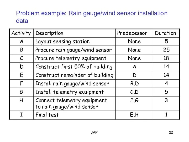
- 22. JAP Problem example: Rain gauge/wind sensor installation data
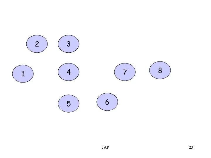
- 23. JAP 1 2 3 4 5 6 7 8
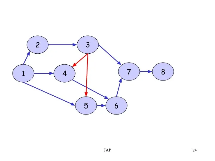
- 24. JAP 1 2 3 4 5 6 7 8
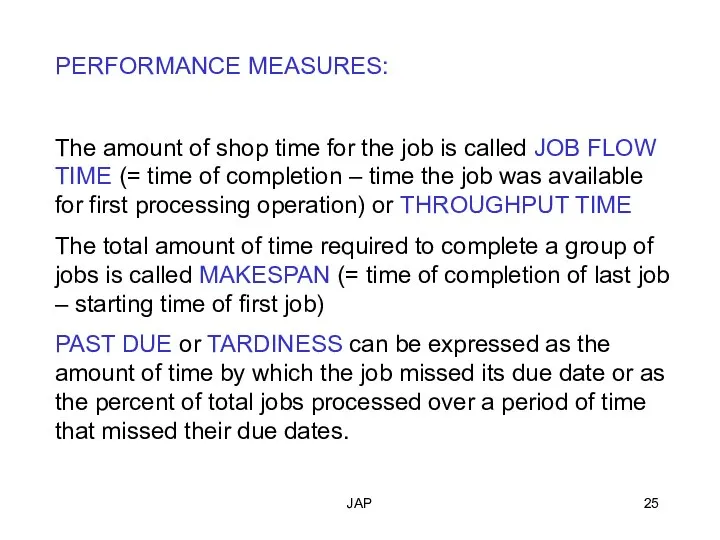
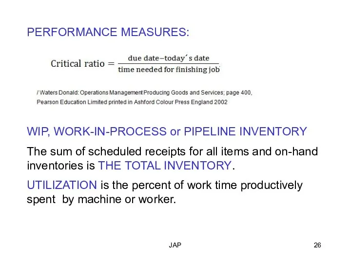
- 25. JAP PERFORMANCE MEASURES: The amount of shop time for the job is called JOB FLOW TIME
- 26. JAP PERFORMANCE MEASURES: WIP, WORK-IN-PROCESS or PIPELINE INVENTORY The sum of scheduled receipts for all items
- 27. JAP Problem of Economic batch quantity? If you consider a factory that needs to produce an
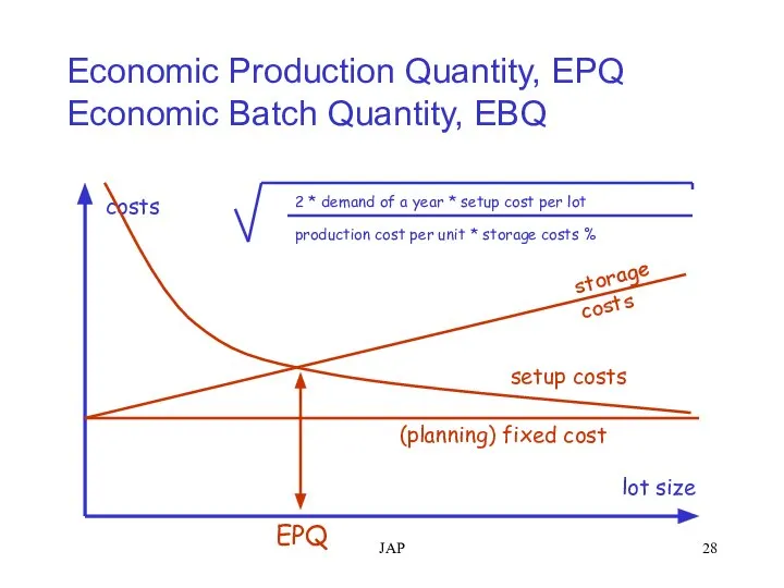
- 28. JAP Economic Production Quantity, EPQ Economic Batch Quantity, EBQ costs lot size (planning) fixed cost storage
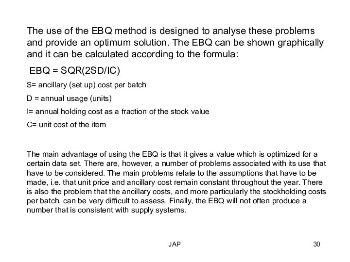
- 29. JAP The costs associated with batch production can be categorized as direct and ancillary. Direct costs
- 30. JAP The use of the EBQ method is designed to analyse these problems and provide an
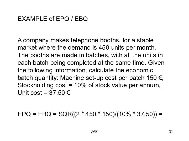
- 31. JAP EXAMPLE of EPQ / EBQ A company makes telephone booths, for a stable market where
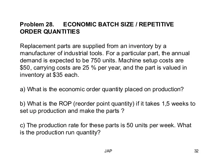
- 32. JAP Problem 28. ECONOMIC BATCH SIZE / REPETITIVE ORDER QUANTITIES Replacement parts are supplied from an
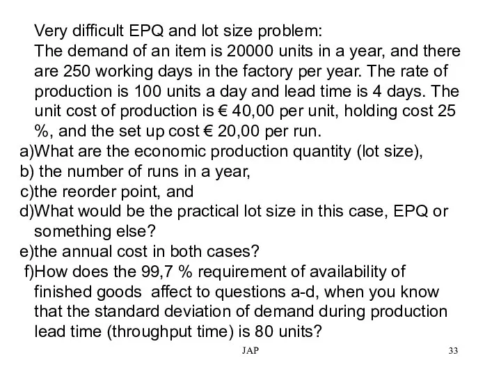
- 33. JAP Very difficult EPQ and lot size problem: The demand of an item is 20000 units
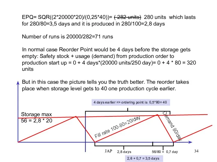
- 34. JAP EPQ= SQR((2*20000*20)/(0,25*40))= ( 282 units) 280 units which lasts for 280/80=3,5 days and it is
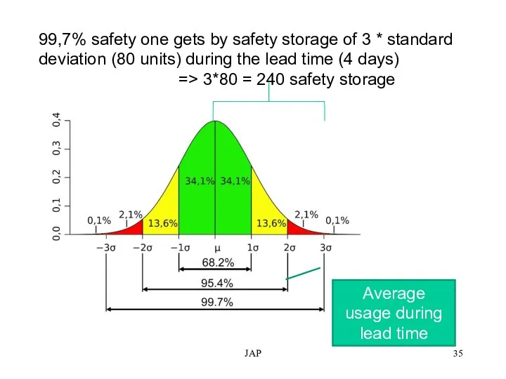
- 35. JAP 99,7% safety one gets by safety storage of 3 * standard deviation (80 units) during
- 36. 85 103 130 127 162 30 88 51 72 32 20 60 105 29 15 40
- 38. Скачать презентацию
JAP
Scheduling means the allocation of resources over time to accomplish specific
JAP
Scheduling means the allocation of resources over time to accomplish specific
JAP
The two basic manufacturing environments are:
A JOB SHOP (Process focused system)
JAP
The two basic manufacturing environments are:
A JOB SHOP (Process focused system)
JAP
Single Processor Scheduling (no alternative routing)
In some cases an entire plant
JAP
Single Processor Scheduling (no alternative routing)
In some cases an entire plant
JAP
Allocate your customers to ABC-classes
A class –strategic customers / most profitable
JAP
Allocate your customers to ABC-classes
A class –strategic customers / most profitable
JAP
Typically scheduling is divided to:
Rough planning - > Master Production
JAP
Typically scheduling is divided to:
Rough planning - > Master Production
JAP
Rough planning – MPS
What are the main objectives, reasoning and
JAP
Rough planning – MPS
What are the main objectives, reasoning and
JAP
TASK 1:
Estimating realistic delivery times
Specially needed for sales – for customer
JAP
TASK 1:
Estimating realistic delivery times
Specially needed for sales – for customer
JAP
TASK 2:
Ensuring the resources needed
Specially needed to keep the delivery time
JAP
TASK 2:
Ensuring the resources needed
Specially needed to keep the delivery time
JAP
TASK 3:
Controlling / managing the work load
Specially needed for production planning
JAP
TASK 3:
Controlling / managing the work load
Specially needed for production planning
JAP
MPS + Bids
JAP
MPS + Bids
JAP
MPS + Bids + probability for order
JAP
MPS + Bids + probability for order
JAP
MPS + Bids + capacity utilization + bid ratio
JAP
MPS + Bids + capacity utilization + bid ratio
JAP
JAP
JAP
Fine Scheduling -> weeks, days, and hours on operation level including
JAP
Fine Scheduling -> weeks, days, and hours on operation level including
JAP
GANTT CHART can be used as a tool for sequencing work
JAP
GANTT CHART can be used as a tool for sequencing work
JAP
A machine chart depicts the sequence of future work at three
JAP
A machine chart depicts the sequence of future work at three
JAP
CRITICAL PATH METHOD (CPM) offers a systematic procedure for selecting the
JAP
CRITICAL PATH METHOD (CPM) offers a systematic procedure for selecting the
G
A
B
E
F
H
C
D
Problem 12a. Critical Path, missing dummy arrow
You have the following list of
G
A
B
E
F
H
C
D
Problem 12a. Critical Path, missing dummy arrow
You have the following list of
JAP
JAP
JAP
JAP
JAP
Problem example: Rain gauge/wind sensor installation data
JAP
Problem example: Rain gauge/wind sensor installation data
JAP
1
2
3
4
5
6
7
8
JAP
1
2
3
4
5
6
7
8
JAP
1
2
3
4
5
6
7
8
JAP
1
2
3
4
5
6
7
8
JAP
PERFORMANCE MEASURES:
The amount of shop time for the job is called
JAP
PERFORMANCE MEASURES:
The amount of shop time for the job is called
JAP
PERFORMANCE MEASURES:
WIP, WORK-IN-PROCESS or PIPELINE INVENTORY
The sum of scheduled receipts
JAP
PERFORMANCE MEASURES:
WIP, WORK-IN-PROCESS or PIPELINE INVENTORY
The sum of scheduled receipts
JAP
Problem of Economic batch quantity?
If you consider a factory that needs
JAP
Problem of Economic batch quantity?
If you consider a factory that needs
JAP
Economic Production Quantity, EPQ
Economic Batch Quantity, EBQ
costs
lot size
(planning) fixed cost
storage costs
setup
JAP
Economic Production Quantity, EPQ
Economic Batch Quantity, EBQ
costs
lot size
(planning) fixed cost
storage costs
setup
JAP
The costs associated with batch production can be categorized as direct
JAP
The costs associated with batch production can be categorized as direct
JAP
The use of the EBQ method is designed to analyse these
JAP
The use of the EBQ method is designed to analyse these
JAP
EXAMPLE of EPQ / EBQ
A company makes telephone booths, for a
JAP
EXAMPLE of EPQ / EBQ
A company makes telephone booths, for a
JAP
Problem 28. ECONOMIC BATCH SIZE / REPETITIVE ORDER QUANTITIES
Replacement parts are
JAP
Problem 28. ECONOMIC BATCH SIZE / REPETITIVE ORDER QUANTITIES
Replacement parts are
JAP
Very difficult EPQ and lot size problem:
The demand of an item
JAP
Very difficult EPQ and lot size problem:
The demand of an item
JAP
EPQ= SQR((2*20000*20)/(0,25*40))= ( 282 units) 280 units which lasts for 280/80=3,5
JAP
EPQ= SQR((2*20000*20)/(0,25*40))= ( 282 units) 280 units which lasts for 280/80=3,5
JAP
99,7% safety one gets by safety storage of 3 * standard
JAP
99,7% safety one gets by safety storage of 3 * standard
85
103
130
127
162
30
88
51
72
32
20
60
105
29
15
40
BEGIN
END
I II III IV
Work Phases
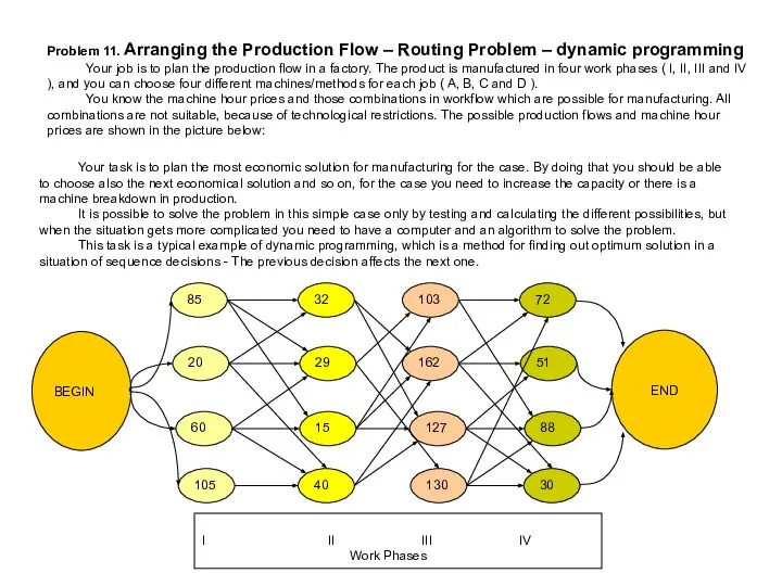
Problem 11. Arranging the Production Flow
85
103
130
127
162
30
88
51
72
32
20
60
105
29
15
40
BEGIN
END
I II III IV
Work Phases
Problem 11. Arranging the Production Flow
 История возникновения контрабанды
 Физиология органа зрения и основные зрительные функции
 Safepay
 Green_Chess_template
 Политическая элита и политическое лидерство
 p53-2
p53-2 Торжественный Вход Господень в Иерусалим
 Русская изба
 Презентация на тему "Клинические испытания новых лекарственных препаратов" - скачать презентации по Медицине
 Государственный мемориальный и природный музей–заповедник И.С. Тургенева «Спасское-Лутовиново»
 Обработка результатов динамических испытаний строительных конструкций
 Мощность и КПД электрических машин
 Меры длины Выполнил ученик 3 Б класса СОШ № 27 города Чебоксары Троешестов Степан
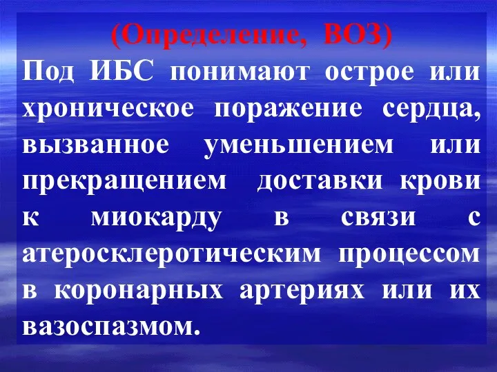 ИБС
ИБС Логистическая цепочка создания стоимости Исаева Катерина Казакова Катя ДС - 07
  Годуновская и строгановская школы иконописи. Искусство парсуны. Симон Ушаков
 День Прикордонних військ України
 Занятие №3. Педагогическая и психологическая оценка уровня образования и развития обучающихся на ступени начального общего об
 Изменчивость и ее формы
 Основные положения экологического права
 автор Позляева Инна Леонидовна МОУ Речицкая средняя школа Московская область
  Ein Besuch auf dem Weihnachtsmarkt
 Хімія металургійних процесів. Теорія сплавів
 Решение задач на движение 4 класс - презентация для начальной школы
 Берёзовоё царство- хорошее лекарство Автор проекта : обучающийся 2 класса Клишин Владислав МОУ «Старосеславинская средняя общ
 Образование и наука в первой половине XIX века
 Разновидности футбола
 ВЛИЯНИЕ ЭКСТРАГЕНИТАЛЬНЫХ ЗАБОЛЕВАНИЙ МАТЕРИ И ВРЕДНЫХ ФАКТОРОВ НА ПЛОД