- Factor Models: Announcements, Surprises, and Expected Returns

Содержание
- 2. 11.1 Factor Models: Announcements, Surprises, and Expected Returns The return on any security consists of two
- 3. 11.1 Factor Models: Announcements, Surprises, and Expected Returns A way to write the return on a
- 4. 11.1 Factor Models: Announcements, Surprises, and Expected Returns Any announcement can be broken down into two
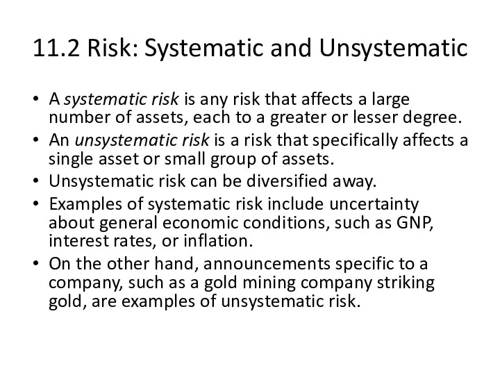
- 5. 11.2 Risk: Systematic and Unsystematic A systematic risk is any risk that affects a large number
- 6. 11.2 Risk: Systematic and Unsystematic Systematic Risk; m Nonsystematic Risk; ε n σ Total risk; U
- 7. 11.2 Risk: Systematic and Unsystematic Systematic risk is referred to as market risk. m influences all
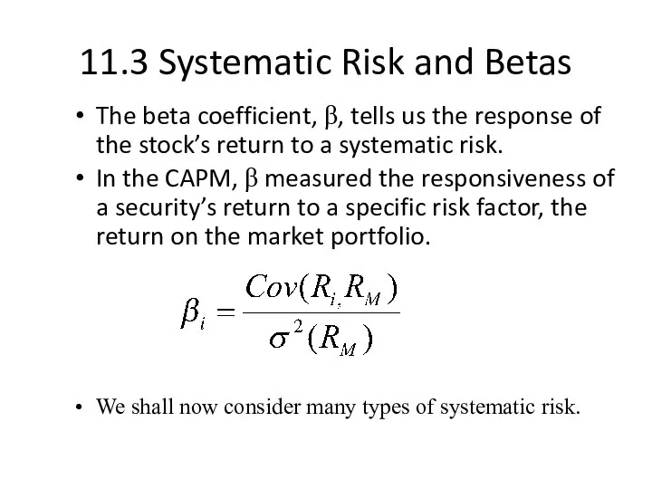
- 8. 11.3 Systematic Risk and Betas The beta coefficient, β, tells us the response of the stock’s
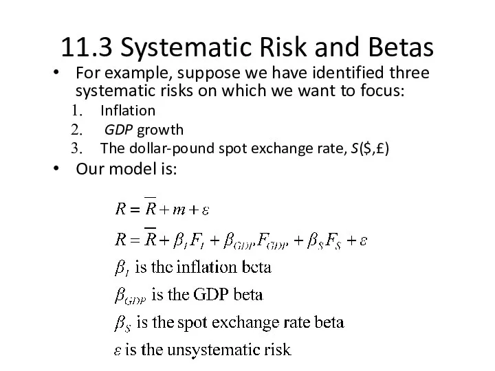
- 9. 11.3 Systematic Risk and Betas For example, suppose we have identified three systematic risks on which
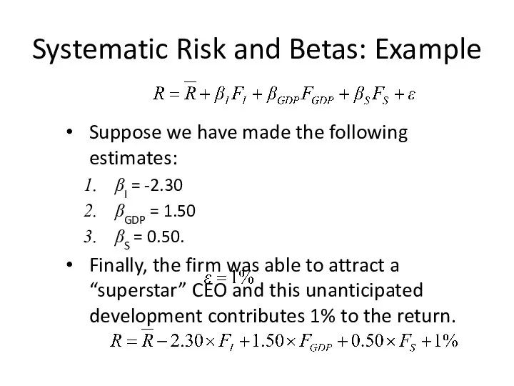
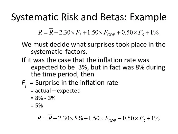
- 10. Systematic Risk and Betas: Example Suppose we have made the following estimates: βI = -2.30 βGDP
- 11. Systematic Risk and Betas: Example We must decide what surprises took place in the systematic factors.
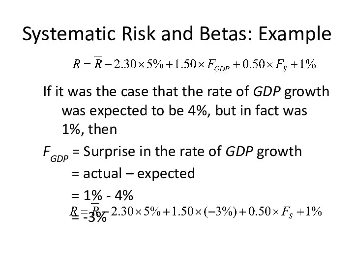
- 12. Systematic Risk and Betas: Example If it was the case that the rate of GDP growth
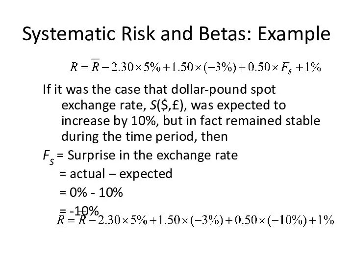
- 13. Systematic Risk and Betas: Example If it was the case that dollar-pound spot exchange rate, S($,£),
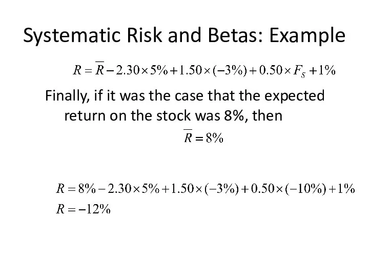
- 14. Systematic Risk and Betas: Example Finally, if it was the case that the expected return on
- 15. 11.4 Portfolios and Factor Models Now let us consider what happens to portfolios of stocks when
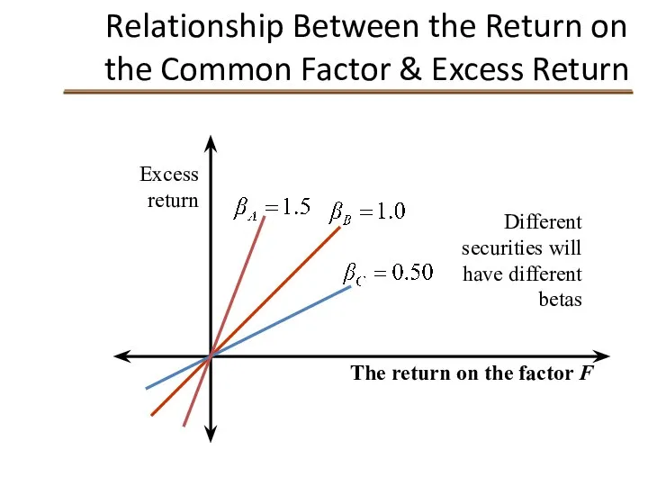
- 16. Relationship Between the Return on the Common Factor & Excess Return Excess return The return on
- 17. Relationship Between the Return on the Common Factor & Excess Return Excess return The return on
- 18. Relationship Between the Return on the Common Factor & Excess Return Excess return The return on
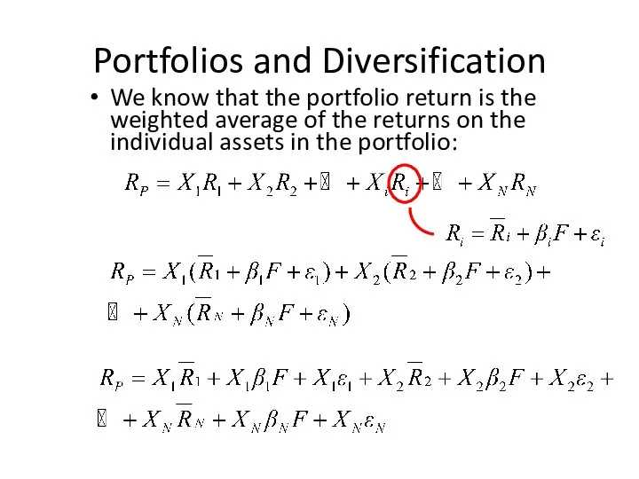
- 19. Portfolios and Diversification We know that the portfolio return is the weighted average of the returns
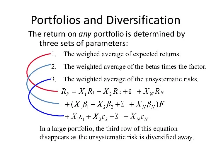
- 20. Portfolios and Diversification The return on any portfolio is determined by three sets of parameters: In
- 21. Portfolios and Diversification So the return on a diversified portfolio is determined by two sets of
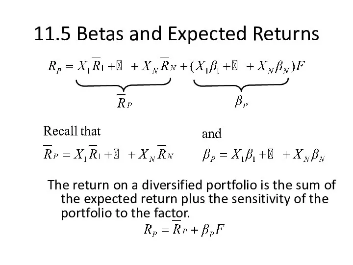
- 22. 11.5 Betas and Expected Returns The return on a diversified portfolio is the sum of the
- 23. Relationship Between β & Expected Return The relevant risk in large and well-diversified portfolios is all
- 24. Relationship Between β & Expected Return Expected return β A B C D SML
- 25. 11.6 The Capital Asset Pricing Model and the Arbitrage Pricing Theory APT applies to well diversified
- 26. Multi-factor APT Example: A Canadian study (Otuteye, CIR 1991) with five factors: the rate of growth
- 27. 11.7 Empirical Approaches to Asset Pricing Both the CAPM and APT are risk-based models. There are
- 29. Скачать презентацию

11.1 Factor Models: Announcements, Surprises, and Expected Returns
The return on any
11.1 Factor Models: Announcements, Surprises, and Expected Returns
The return on any

11.1 Factor Models: Announcements, Surprises, and Expected Returns
A way to write
11.1 Factor Models: Announcements, Surprises, and Expected Returns
A way to write

11.1 Factor Models: Announcements, Surprises, and Expected Returns
Any announcement can be
11.1 Factor Models: Announcements, Surprises, and Expected Returns
Any announcement can be
11.2 Risk: Systematic and Unsystematic
A systematic risk is any risk that
11.2 Risk: Systematic and Unsystematic
A systematic risk is any risk that

11.2 Risk: Systematic and Unsystematic
Systematic Risk; m
Nonsystematic Risk; ε
n
σ
Total risk;
11.2 Risk: Systematic and Unsystematic
Systematic Risk; m
Nonsystematic Risk; ε
n
σ
Total risk;

11.2 Risk: Systematic and Unsystematic
Systematic risk is referred to as market
11.2 Risk: Systematic and Unsystematic
Systematic risk is referred to as market
11.3 Systematic Risk and Betas
The beta coefficient, β, tells us the
11.3 Systematic Risk and Betas
The beta coefficient, β, tells us the
11.3 Systematic Risk and Betas
For example, suppose we have identified three
11.3 Systematic Risk and Betas
For example, suppose we have identified three
Systematic Risk and Betas: Example
Suppose we have made the following estimates:
βI
Systematic Risk and Betas: Example
Suppose we have made the following estimates:
βI
Systematic Risk and Betas: Example
We must decide what surprises took place
Systematic Risk and Betas: Example
We must decide what surprises took place
Systematic Risk and Betas: Example
If it was the case that the
Systematic Risk and Betas: Example
If it was the case that the
Systematic Risk and Betas: Example
If it was the case that dollar-pound
Systematic Risk and Betas: Example
If it was the case that dollar-pound
Systematic Risk and Betas: Example
Finally, if it was the case that
Systematic Risk and Betas: Example
Finally, if it was the case that

11.4 Portfolios and Factor Models
Now let us consider what happens to
11.4 Portfolios and Factor Models
Now let us consider what happens to

Relationship Between the Return on the Common Factor & Excess Return
Excess
Relationship Between the Return on the Common Factor & Excess Return
Excess

Relationship Between the Return on the Common Factor & Excess Return
Excess
Relationship Between the Return on the Common Factor & Excess Return
Excess
Relationship Between the Return on the Common Factor & Excess Return
Excess
Relationship Between the Return on the Common Factor & Excess Return
Excess
Portfolios and Diversification
We know that the portfolio return is the weighted
Portfolios and Diversification
We know that the portfolio return is the weighted
Portfolios and Diversification
The return on any portfolio is determined by three
Portfolios and Diversification
The return on any portfolio is determined by three

Portfolios and Diversification
So the return on a diversified portfolio is determined
Portfolios and Diversification
So the return on a diversified portfolio is determined
11.5 Betas and Expected Returns
The return on a diversified portfolio is
11.5 Betas and Expected Returns
The return on a diversified portfolio is

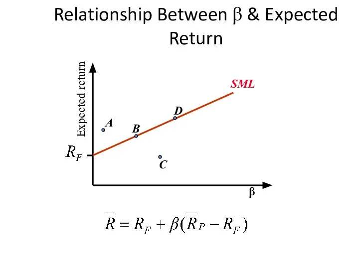
Relationship Between β & Expected Return
The relevant risk in large and
Relationship Between β & Expected Return
The relevant risk in large and
Relationship Between β & Expected Return
Expected return
β
A
B
C
D
SML
Relationship Between β & Expected Return
Expected return
β
A
B
C
D
SML

11.6 The Capital Asset Pricing Model and the Arbitrage Pricing Theory
APT
11.6 The Capital Asset Pricing Model and the Arbitrage Pricing Theory
APT
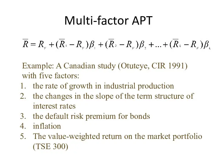
Multi-factor APT
Example: A Canadian study (Otuteye, CIR 1991)
with five factors:
the rate
Multi-factor APT
Example: A Canadian study (Otuteye, CIR 1991)
with five factors:
the rate

11.7 Empirical Approaches to Asset Pricing
Both the CAPM and APT are
11.7 Empirical Approaches to Asset Pricing
Both the CAPM and APT are
 Ընդհանուր պատկերացումներ տնտեսության մասին
 Елдердің экономикалық көшбасшылары. Елдер түрлері: орталық, жартылай перифериялы, перифериялы. Географиялық орталықтар
 Актуальные вопросы туризма в России
 Квалиметрия. Техника применения экспертного метода измерения качества продукции
 Политические институты и экономические результаты
 Безработица. Типы и формы безработицы
 Экономикалық теорияның пәні және әдістері
 История становления предпринимательства в России
 Пятиэтапная модель Роберта Гранта. GAP-анализ
 Малиновский район міста Одеси. Слайды
 Содержание дисциплины Экономика и ее задачи
 Роль иностранного капитала в экономике России XIX-XX веков
 Мировое хозяйство и международная торговля
 Экономика - искусство ведения хозяйства
 Типы экономических систем
 Внешнеэкономическая деятельность Торгово-промышленной палаты Российской Федерации
 Основи аналізу попиту
 Customer behavior specifics in the access economy: comparison of Russian and Italian carsharing customers
 Презентация Таможенная политика в период складывания единого централизованного государства.
 Планирование производственных процессов и определение состава машинно-тракторного парка в ООО «Милославский ячмень»
 Еколого-економічне обґрунтування структури угідь та організації сівозмін фермерського господарства
 Поддорское сельское поселение. Проект поддержки местных инициатив
 Организационная структура отрасли «торговля»
 Рынки факторов производства Цель: изучить специфику факторных рынков
 ВТО
ВТО Процедура взаимодействия СК с поставщиками по сервису (Мониторинг KPI и производственный аудит)
 Нарықтық экономикалық жүйе және нарықтық механизм
 Анализ региона: Юго-Восточная Азия