- General equilibrium in the open (trading) economy

Содержание
- 2. Topic 2. General equilibrium in the open (trading) economy 2.1. General equilibrium conditions in the open
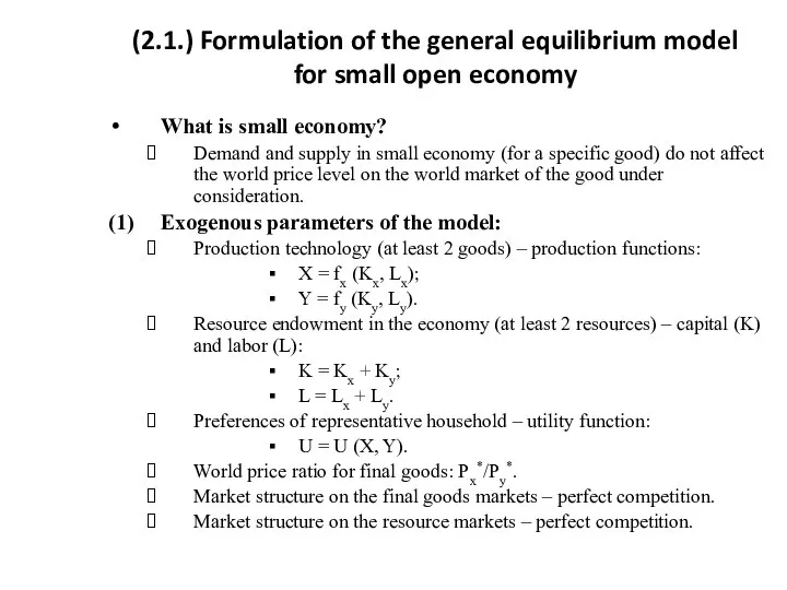
- 3. (2.1.) Formulation of the general equilibrium model for small open economy What is small economy? Demand
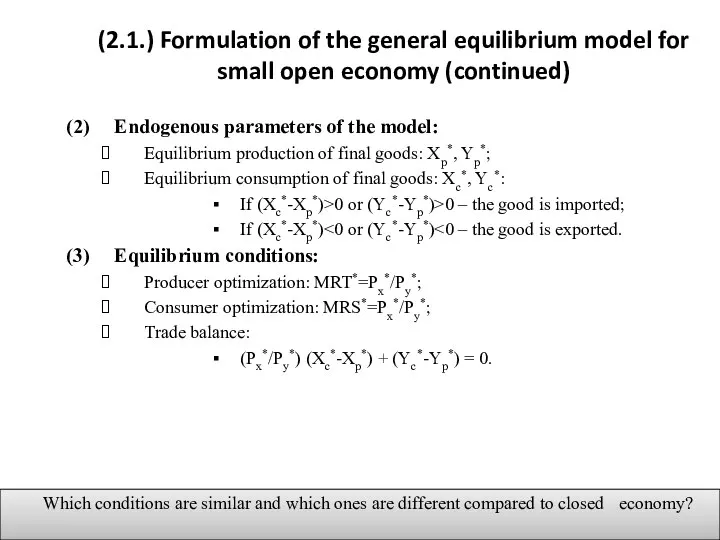
- 4. (2.1.) Formulation of the general equilibrium model for small open economy (continued) (2) Endogenous parameters of
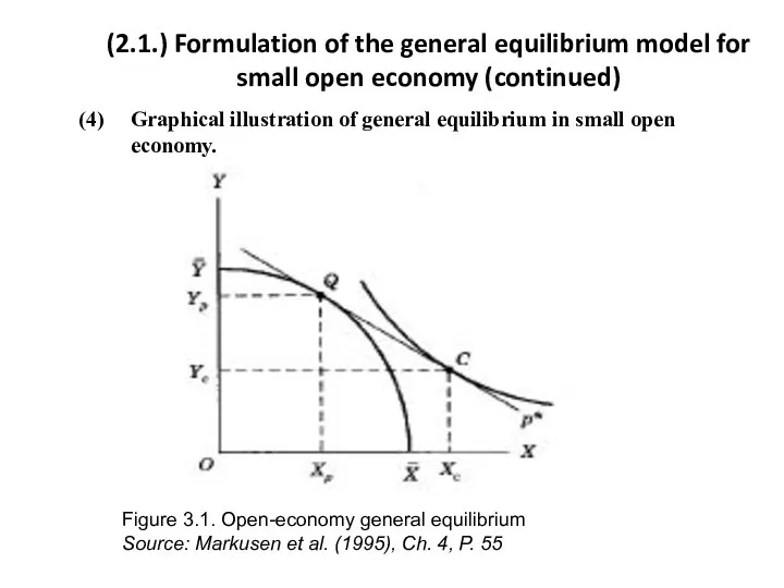
- 5. (2.1.) Formulation of the general equilibrium model for small open economy (continued) (4) Graphical illustration of
- 6. (2.2.) The concept of the excess demand function Definition (general): The excess demand function: relates the
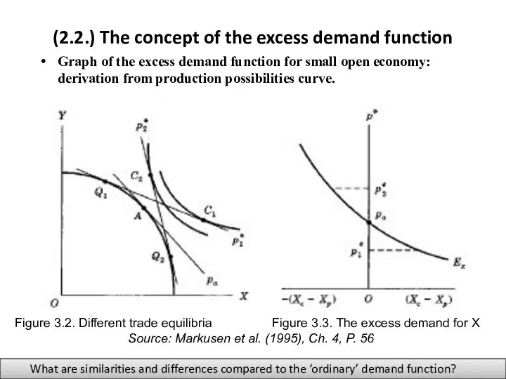
- 7. (2.2.) The concept of the excess demand function Graph of the excess demand function for small
- 8. (2.2.) The concept of the excess demand function Graph of the excess demand function for small
- 9. (2.3.) Conditions of international general equilibrium Which economies form the world economy? Large economies (at least
- 10. (2.3.) Conditions of international general equilibrium (continued) (2) Endogenous parameters of the model: Equilibrium production of
- 11. (2.3.) Conditions of international general equilibrium (continued) (4) Graphical illustration of general equilibrium in the world
- 12. (2.3.) Conditions of international general equilibrium (continued) (4) Graphical illustration of general equilibrium in the world
- 13. Exercise session 2 (2) Think about topics for reports during exercise sessions and work on a
- 15. Скачать презентацию

Topic 2. General equilibrium in the open (trading) economy
2.1. General equilibrium
Topic 2. General equilibrium in the open (trading) economy
2.1. General equilibrium
(2.1.) Formulation of the general equilibrium model
for small open economy
What
(2.1.) Formulation of the general equilibrium model
for small open economy
What
(2.1.) Formulation of the general equilibrium model for small open economy
(2.1.) Formulation of the general equilibrium model for small open economy
(2.1.) Formulation of the general equilibrium model for small open economy
(2.1.) Formulation of the general equilibrium model for small open economy
(2.2.) The concept of the excess demand function
Definition (general):
The excess
(2.2.) The concept of the excess demand function
Definition (general):
The excess
(2.2.) The concept of the excess demand function
Graph of the
(2.2.) The concept of the excess demand function
Graph of the
(2.2.) The concept of the excess demand function
Graph of the
(2.2.) The concept of the excess demand function
Graph of the
(2.3.) Conditions of international general equilibrium
Which economies form the world economy?
Large
(2.3.) Conditions of international general equilibrium
Which economies form the world economy?
Large

(2.3.) Conditions of international general equilibrium (continued)
(2) Endogenous parameters of the model:
Equilibrium
(2.3.) Conditions of international general equilibrium (continued)
(2) Endogenous parameters of the model:
Equilibrium

(2.3.) Conditions of international general equilibrium (continued)
(4) Graphical illustration of general equilibrium
(2.3.) Conditions of international general equilibrium (continued)
(4) Graphical illustration of general equilibrium
(2.3.) Conditions of international general equilibrium (continued)
(4) Graphical illustration of general equilibrium
(2.3.) Conditions of international general equilibrium (continued)
(4) Graphical illustration of general equilibrium
Exercise session 2
(2) Think about topics for reports during exercise sessions
(2) Think about topics for reports during exercise sessions
 Экономическая эффективность природоохранной деятельности
 Қоғамдық өндіріс негіздері
 Инновации и инновационная деятельность
 Человеческий капитал ТЭК. Роль ТЭК в экономике страны
 Системный анализ в экономике. Предмет, содержание и задачи курса. Система и ее свойства
 Развитие неоклассической теории (микроэкономика) в 20 – 40 годы ХХ века
 Рыноктық механизмді
 Предложение. Закон предложения
 Безробіття в Україні
 Теория потребительского поведения
 Дефлятор ВВП як показник рівня цін
 Міжнародна безпека. Лекція 5. Економічна безпека та її роль в розвитку світового господарства та МЕВ
 Экономика. Часть 2. Задачи
 Петрозаводск - исполнение поручений
 Эконометрика, начальный курс
 Кредитный потребительский кооператив
 Спрос. Закон спроса. Эластичность спроса
 Құрылыстың сметалық құны
 Экономикалық дамудың үлгілері
 Теория организации. Предприятие в рыночной экономике. Предприятие и его место в системе народного хозяйства. (Часть 2.1.1)
 Проблемы эффективного формирования и использования капитала фирмы
 Методология неоклассической школы
 Состояние и обзор качества товарной продукции, поступившей из КНР на территорию Республики Хакасия
 Валютное регулирование и валютный контроль. Лекция 3 - Роль валютного регулирования в микро- и макроэкономике
 Концепція розвитку велосипедної інфраструктури міста Южноукраїнська
 Марксистская (материалистическая) теория
 Корпоративная социальная ответственность
 Використання електричної енергії в Україні