- Monopoly Behavior

Содержание
- 2. A Scotsman phones a dentist to inquire about the cost for a tooth extraction : —
- 3. — "I can't guarantee their professionalism and it'll be painful. But the price could drop by
- 4. How Should a Monopoly Price? So far a monopoly has been thought of as a firm
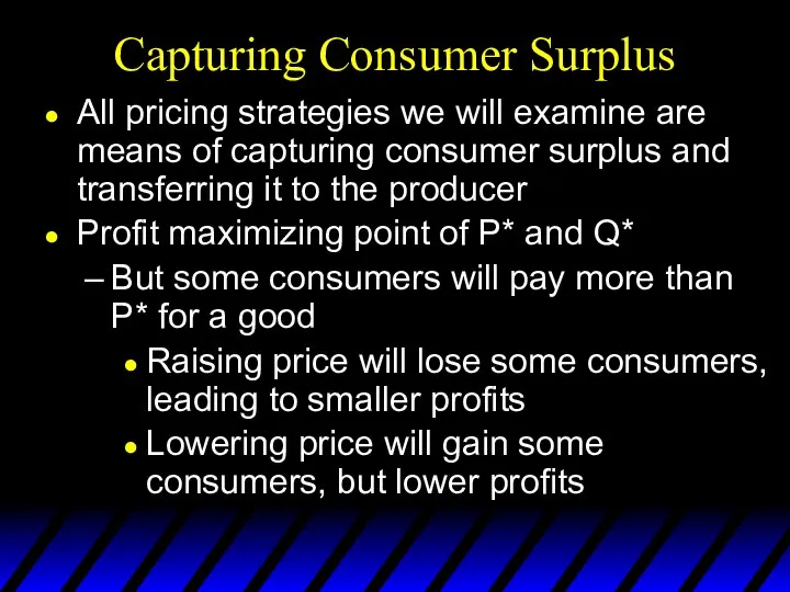
- 5. Capturing Consumer Surplus All pricing strategies we will examine are means of capturing consumer surplus and
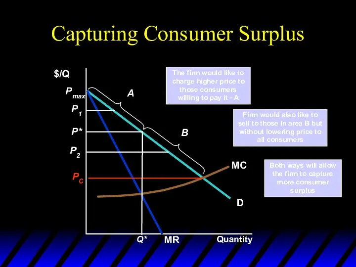
- 6. Capturing Consumer Surplus Quantity $/Q The firm would like to charge higher price to those consumers
- 7. Capturing Consumer Surplus Price discrimination is the practice of charging different prices to different consumers for
- 8. Price discrimination Price discrimination requires the absence of resale
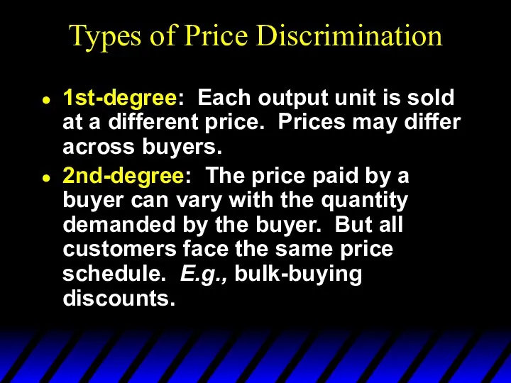
- 9. Types of Price Discrimination 1st-degree: Each output unit is sold at a different price. Prices may
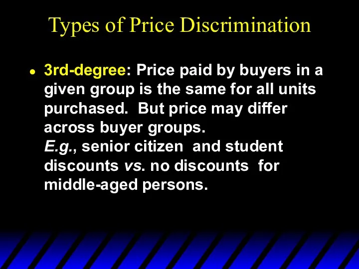
- 10. Types of Price Discrimination 3rd-degree: Price paid by buyers in a given group is the same
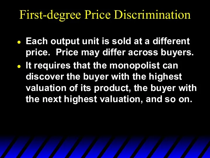
- 11. First-degree Price Discrimination Each output unit is sold at a different price. Price may differ across
- 12. First-degree Price Discrimination p(y) y $/output unit MC(y) Sell the th unit for $
- 13. First-degree Price Discrimination p(y) y $/output unit MC(y) Sell the th unit for $ Later on
- 14. First-degree Price Discrimination p(y) y $/output unit MC(y) Sell the th unit for $ Later on
- 15. First-degree Price Discrimination p(y) y $/output unit MC(y) The gains to the monopolist on these trades
- 16. First-degree Price Discrimination p(y) y $/output unit MC(y) So the sum of the gains to the
- 17. First-degree Price Discrimination p(y) y $/output unit MC(y) The monopolist gets the maximum possible gains from
- 18. Fig. 25.2
- 19. First-degree Price Discrimination First-degree price discrimination gives a monopolist all of the possible gains-to-trade, leaves the
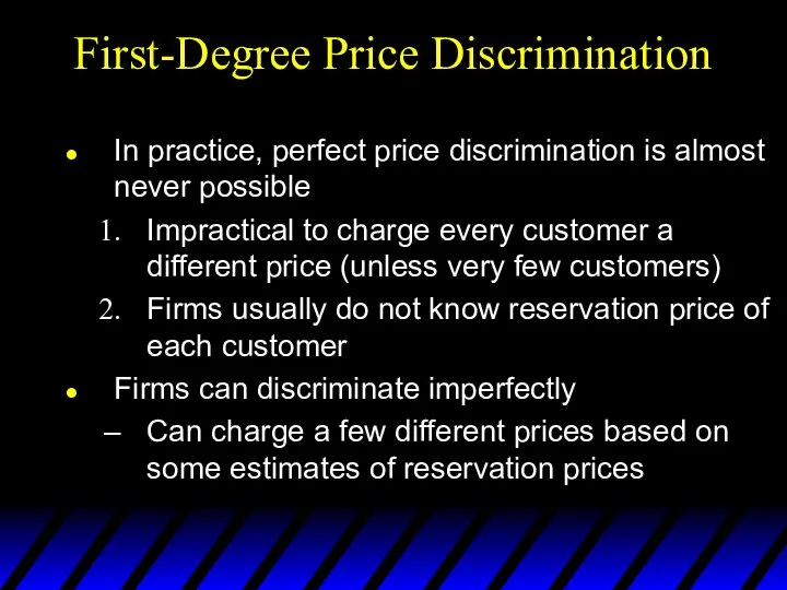
- 20. First-Degree Price Discrimination In practice, perfect price discrimination is almost never possible Impractical to charge every
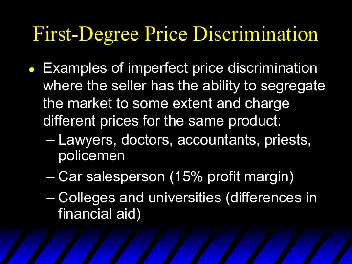
- 21. First-Degree Price Discrimination Examples of imperfect price discrimination where the seller has the ability to segregate
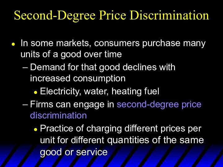
- 22. Second-Degree Price Discrimination In some markets, consumers purchase many units of a good over time Demand
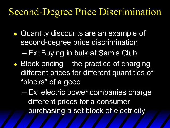
- 23. Second-Degree Price Discrimination Quantity discounts are an example of second-degree price discrimination Ex: Buying in bulk
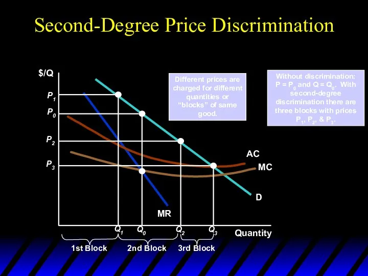
- 24. Second-Degree Price Discrimination $/Q Without discrimination: P = P0 and Q = Q0. With second-degree discrimination
- 25. Fig. 25.3 Second-Degree Price Discrimination Self selection
- 26. Fig. 25.3 Second-Degree Price Discrimination Self selection
- 27. Fig. 25.3 Second-Degree Price Discrimination Self selection
- 28. Fig. 25.3 Second-Degree Price Discrimination Self selection In practice, the monopolist often encourages self-selection by adjusting
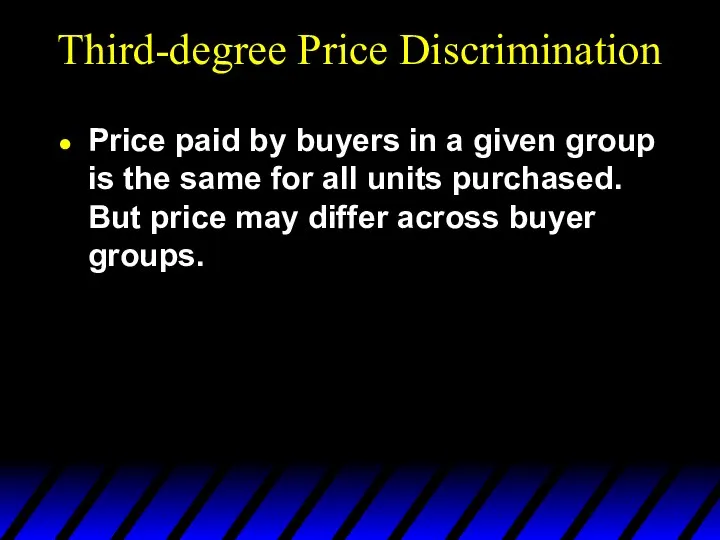
- 29. Third-degree Price Discrimination Price paid by buyers in a given group is the same for all
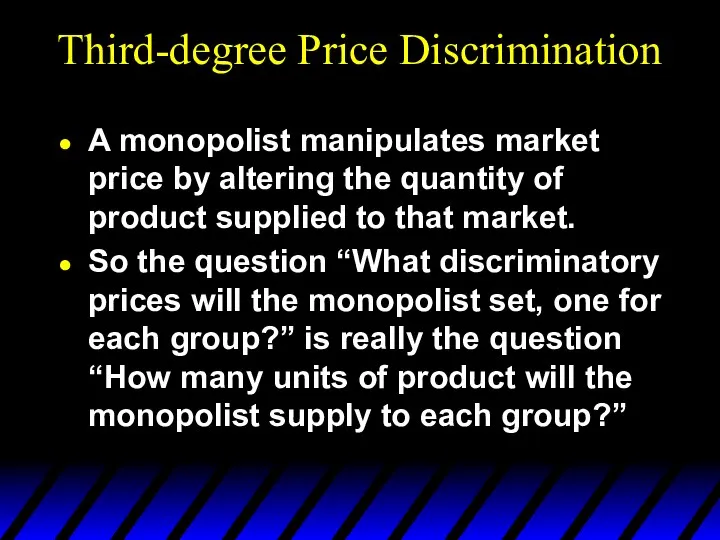
- 30. Third-degree Price Discrimination A monopolist manipulates market price by altering the quantity of product supplied to
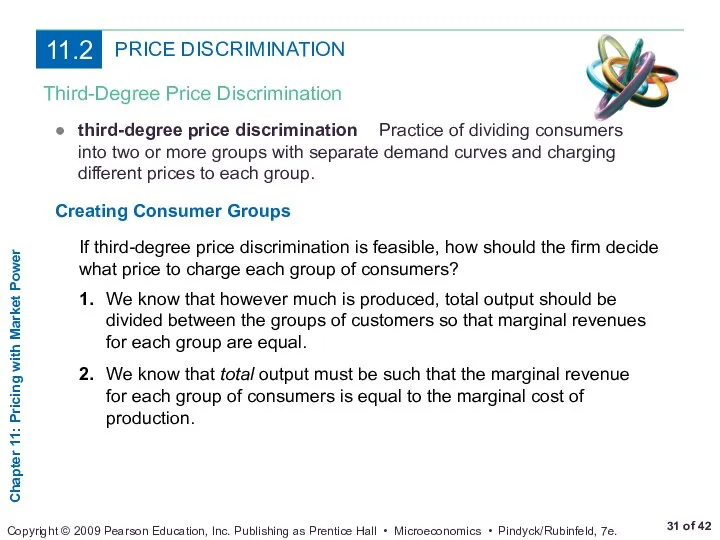
- 31. PRICE DISCRIMINATION Third-Degree Price Discrimination ● third-degree price discrimination Practice of dividing consumers into two or
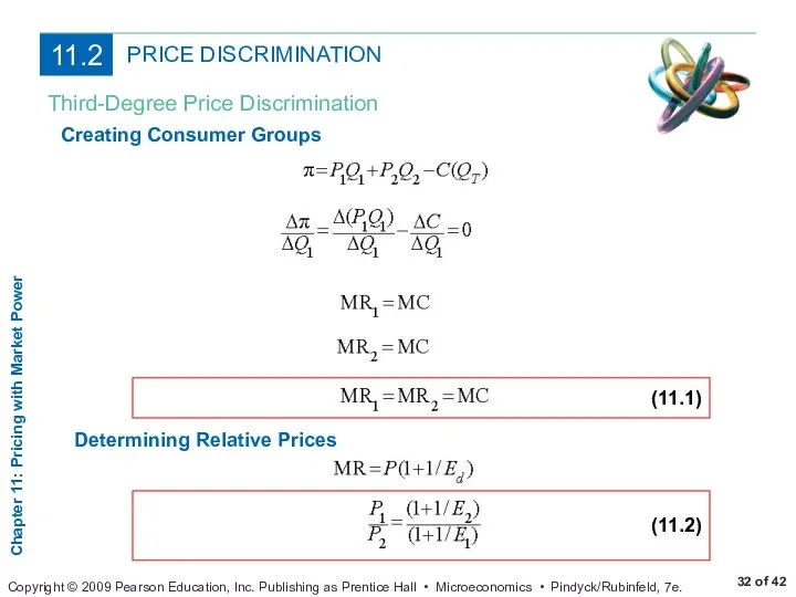
- 32. PRICE DISCRIMINATION Third-Degree Price Discrimination Creating Consumer Groups Determining Relative Prices
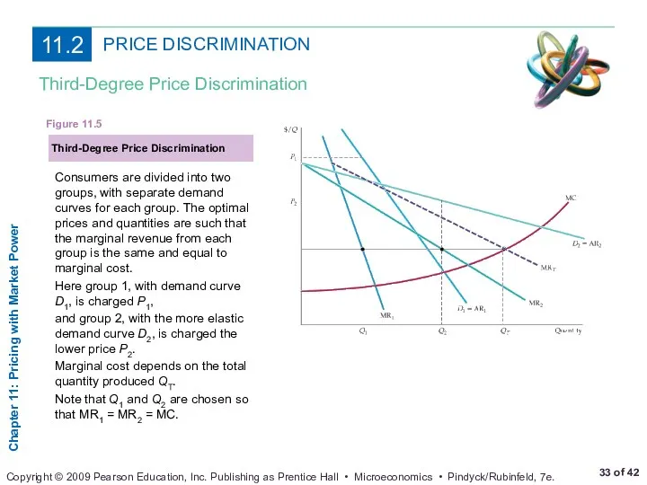
- 33. PRICE DISCRIMINATION Third-Degree Price Discrimination Third-Degree Price Discrimination Figure 11.5 Consumers are divided into two groups,
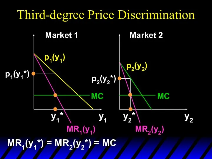
- 34. Third-degree Price Discrimination MR1(y1) MR2(y2) y1 y2 y1* y2* p1(y1*) p2(y2*) MC MC p1(y1) p2(y2) Market
- 35. Third-degree Price Discrimination MR1(y1) MR2(y2) y1 y2 y1* y2* p1(y1*) p2(y2*) MC MC p1(y1) p2(y2) Market
- 36. Third-degree Price Discrimination In which market will the monopolist cause the higher price?
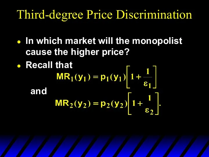
- 37. Third-degree Price Discrimination In which market will the monopolist cause the higher price? Recall that and
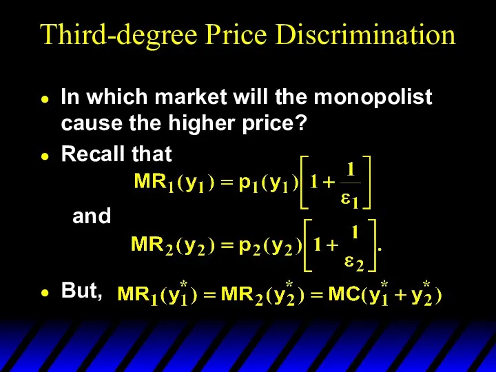
- 38. Third-degree Price Discrimination In which market will the monopolist cause the higher price? Recall that But,
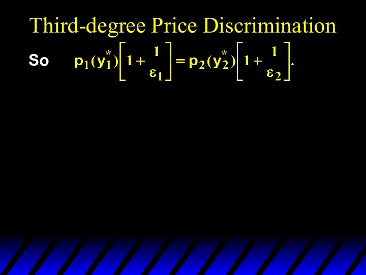
- 39. Third-degree Price Discrimination So
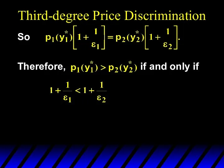
- 40. Third-degree Price Discrimination So Therefore, if and only if
- 41. Third-degree Price Discrimination So Therefore, if and only if
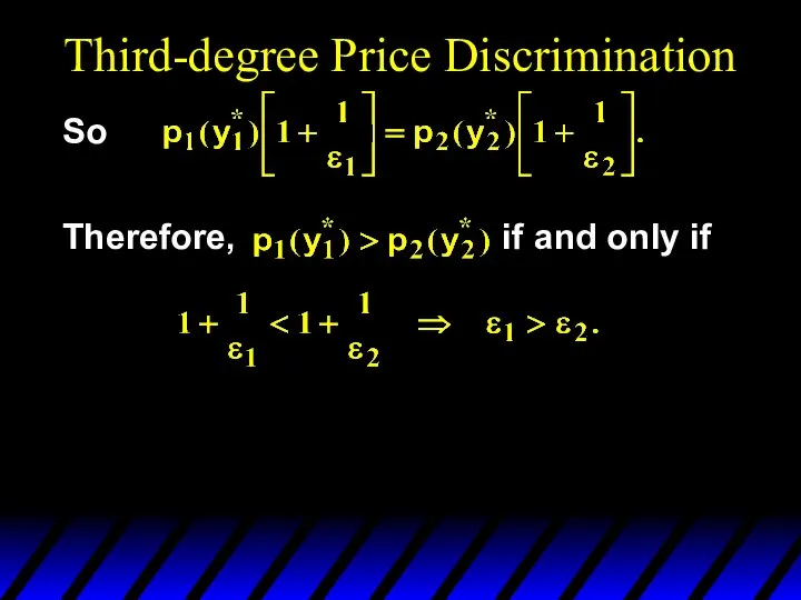
- 42. Third-degree Price Discrimination So Therefore, if and only if The monopolist sets the higher price in
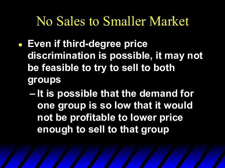
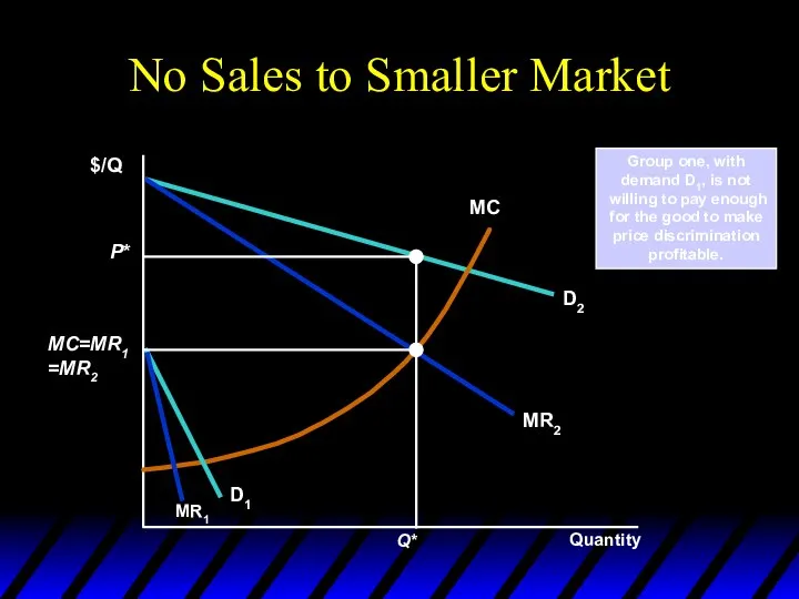
- 43. No Sales to Smaller Market Even if third-degree price discrimination is possible, it may not be
- 44. No Sales to Smaller Market Quantity $/Q Group one, with demand D1, is not willing to
- 45. The Economics of Coupons and Rebates Those consumers who are more price elastic will tend to
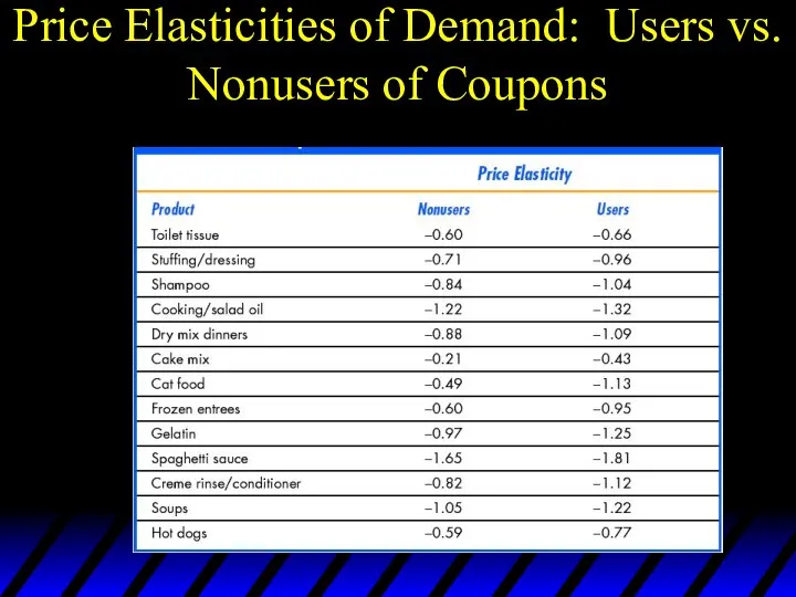
- 46. The Economics of Coupons and Rebates About 20 – 30% of consumers use coupons or rebates
- 47. Price Elasticities of Demand: Users vs. Nonusers of Coupons
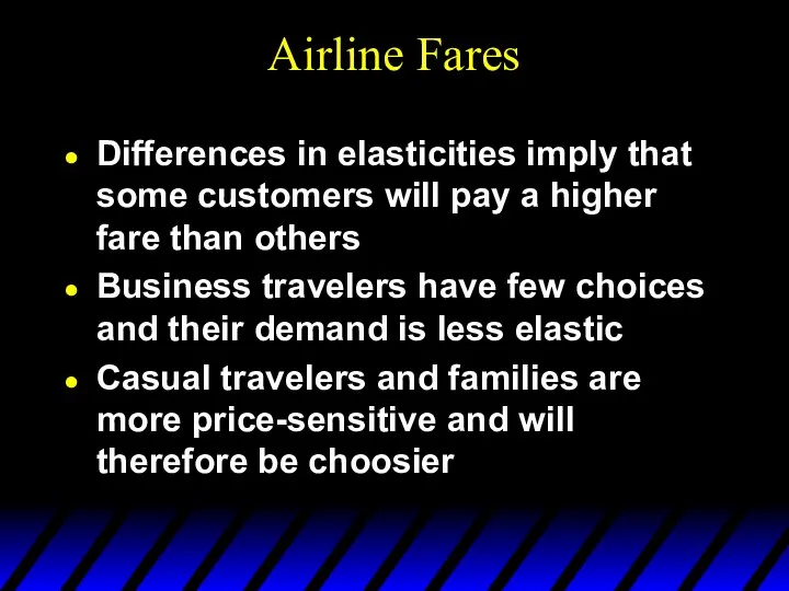
- 48. Airline Fares Differences in elasticities imply that some customers will pay a higher fare than others
- 49. Elasticities of Demand for Air Travel
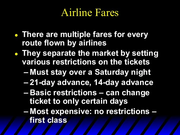
- 50. Airline Fares There are multiple fares for every route flown by airlines They separate the market
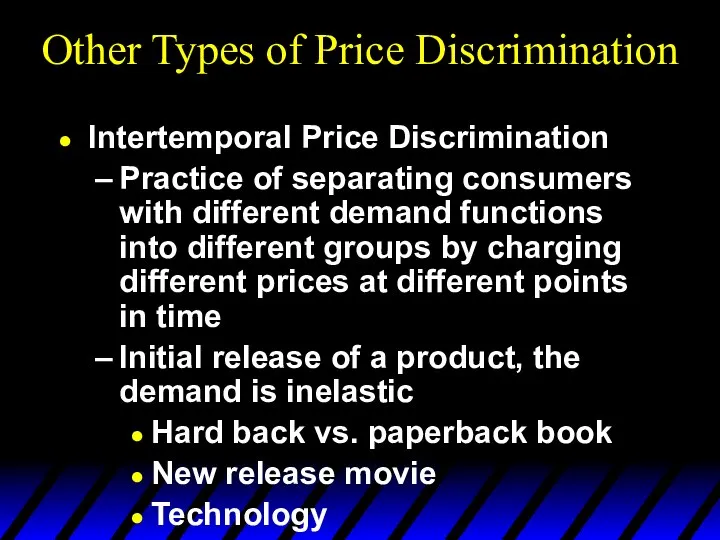
- 51. Other Types of Price Discrimination Intertemporal Price Discrimination Practice of separating consumers with different demand functions
- 52. Intertemporal Price Discrimination Once this market has yielded a maximum profit, firms lower the price to
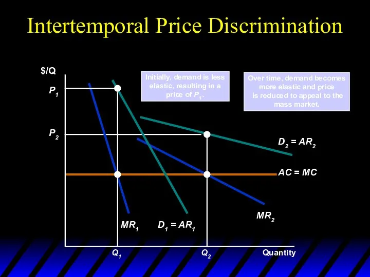
- 53. Intertemporal Price Discrimination Quantity $/Q Over time, demand becomes more elastic and price is reduced to
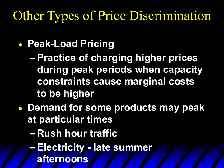
- 54. Other Types of Price Discrimination Peak-Load Pricing Practice of charging higher prices during peak periods when
- 55. Peak-Load Pricing Objective is to increase efficiency by charging customers close to marginal cost Increased MR
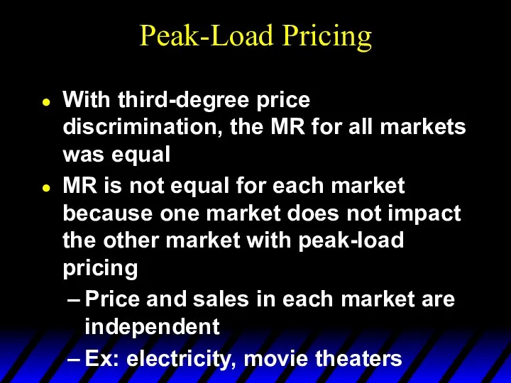
- 56. Peak-Load Pricing With third-degree price discrimination, the MR for all markets was equal MR is not
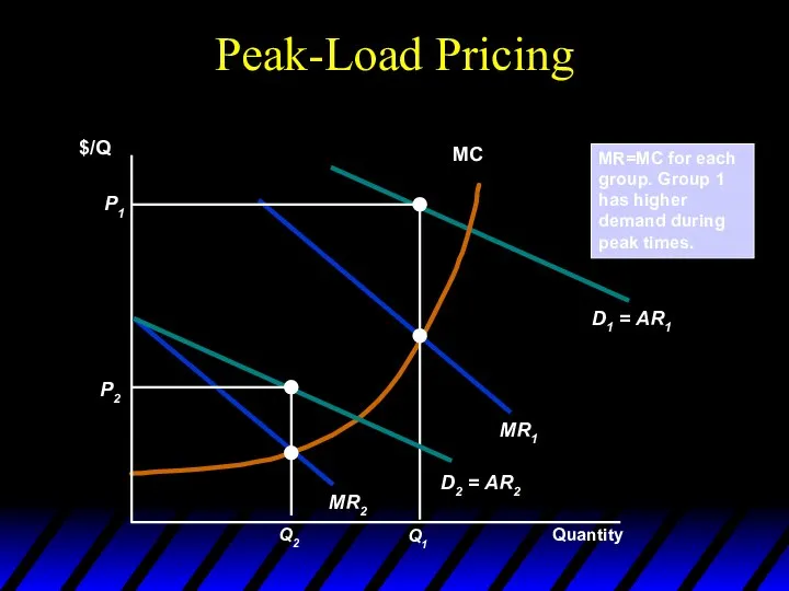
- 57. Peak-Load Pricing Quantity $/Q MR=MC for each group. Group 1 has higher demand during peak times.
- 58. How to Price a Best-Selling Novel How would you arrive at the price for the initial
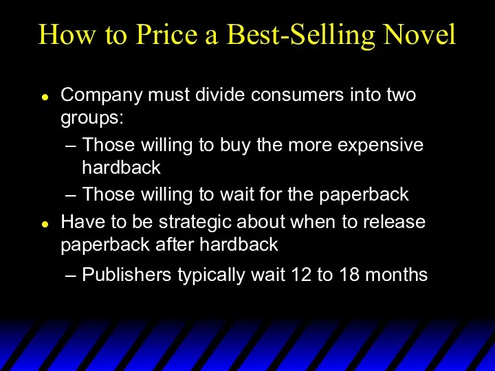
- 59. How to Price a Best-Selling Novel Company must divide consumers into two groups: Those willing to
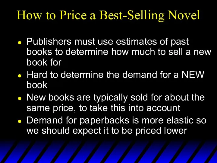
- 60. How to Price a Best-Selling Novel Publishers must use estimates of past books to determine how
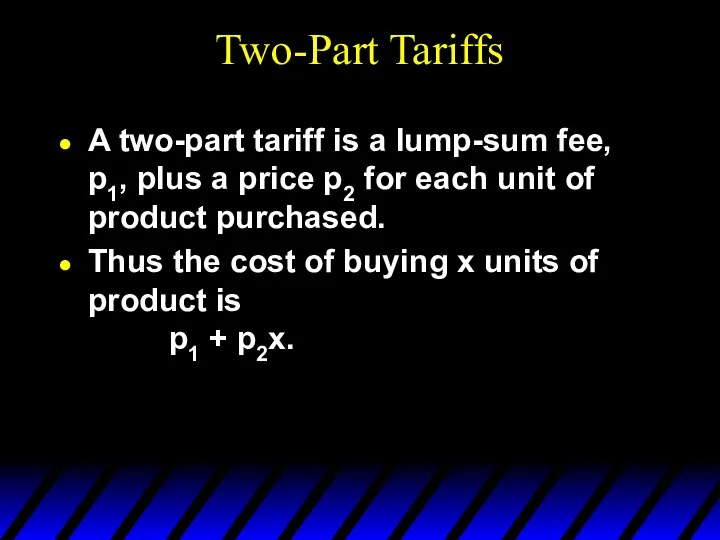
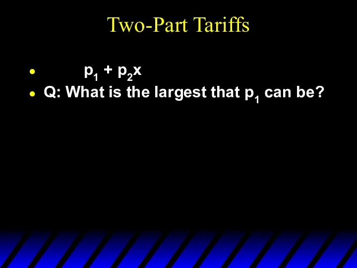
- 61. Two-Part Tariffs A two-part tariff is a lump-sum fee, p1, plus a price p2 for each
- 62. Two-Part Tariffs Should a monopolist prefer a two-part tariff to uniform pricing, or to any of
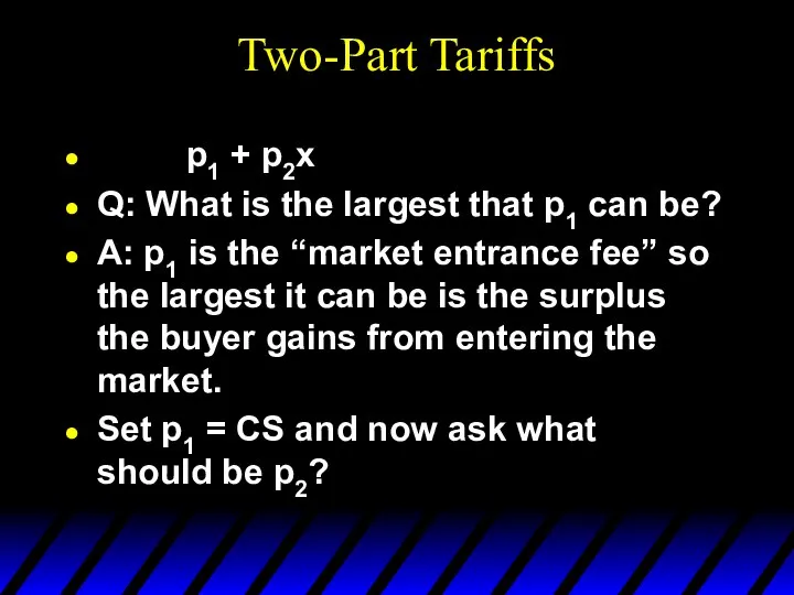
- 63. Two-Part Tariffs p1 + p2x Q: What is the largest that p1 can be?
- 64. Two-Part Tariffs p1 + p2x Q: What is the largest that p1 can be? A: p1
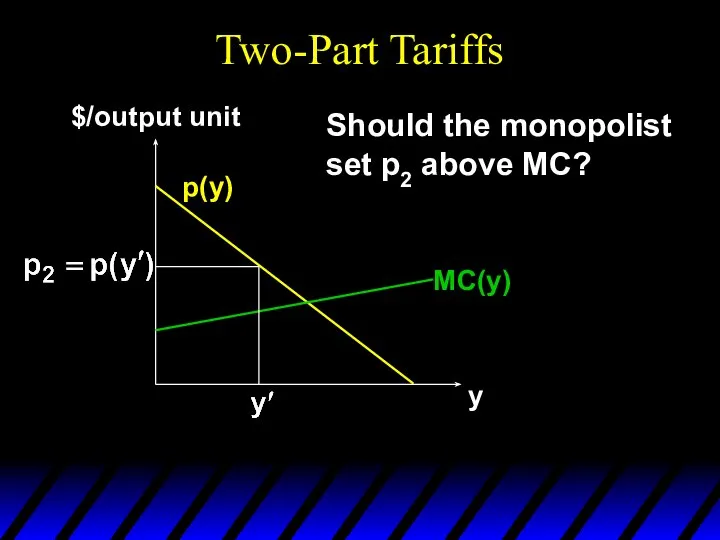
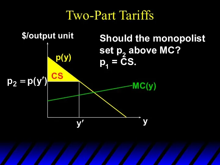
- 65. Two-Part Tariffs p(y) y $/output unit MC(y) Should the monopolist set p2 above MC?
- 66. Two-Part Tariffs p(y) y $/output unit CS Should the monopolist set p2 above MC? p1 =
- 67. Two-Part Tariffs p(y) y $/output unit CS Should the monopolist set p2 above MC? p1 =
- 68. Two-Part Tariffs p(y) y $/output unit CS Should the monopolist set p2 above MC? p1 =
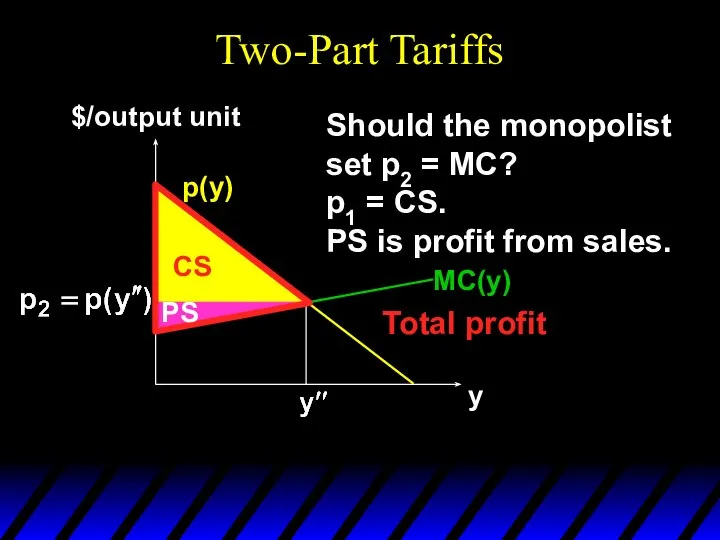
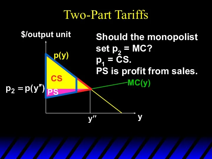
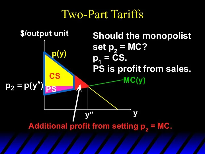
- 69. Two-Part Tariffs p(y) y $/output unit Should the monopolist set p2 = MC? MC(y)
- 70. Two-Part Tariffs p(y) y $/output unit Should the monopolist set p2 = MC? p1 = CS.
- 71. Two-Part Tariffs p(y) y $/output unit Should the monopolist set p2 = MC? p1 = CS.
- 72. Two-Part Tariffs p(y) y $/output unit Should the monopolist set p2 = MC? p1 = CS.
- 73. Two-Part Tariffs p(y) y $/output unit Should the monopolist set p2 = MC? p1 = CS.
- 74. Two-Part Tariffs p(y) y $/output unit Should the monopolist set p2 = MC? p1 = CS.
- 75. Two-Part Tariffs The monopolist maximizes its profit when using a two-part tariff by setting its per
- 76. Two-Part Tariffs A profit-maximizing two-part tariff gives an efficient market outcome in which the monopolist obtains
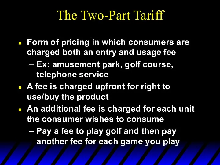
- 77. The Two-Part Tariff Form of pricing in which consumers are charged both an entry and usage
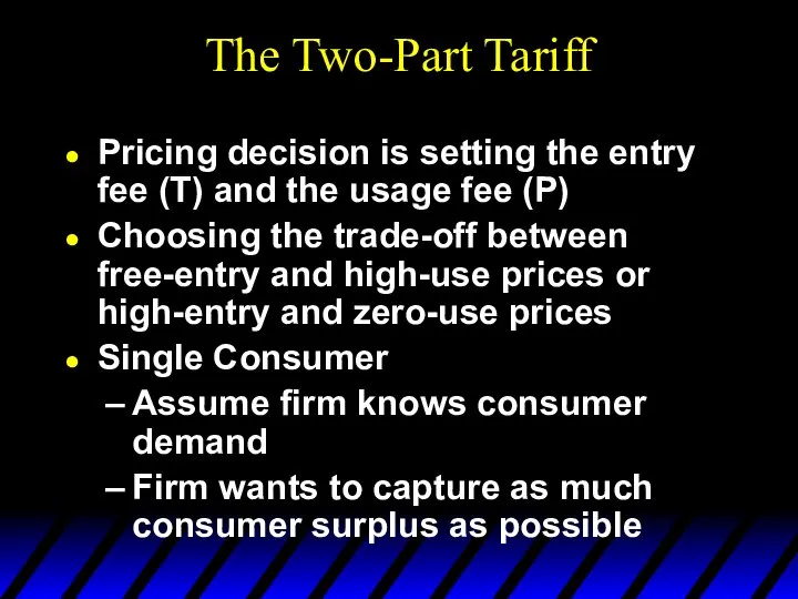
- 78. The Two-Part Tariff Pricing decision is setting the entry fee (T) and the usage fee (P)
- 79. Usage price P* is set equal to MC. Entry price T* is equal to the entire
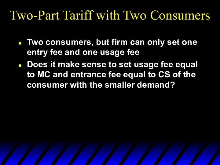
- 80. Two-Part Tariff with Two Consumers Two consumers, but firm can only set one entry fee and
- 81. The price, P*, will be greater than MC. Set T* at the surplus value of D2.
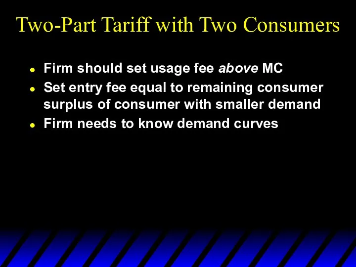
- 82. Two-Part Tariff with Two Consumers Firm should set usage fee above MC Set entry fee equal
- 83. The Two-Part Tariff with Many Consumers No exact way to determine P* and T* Must consider
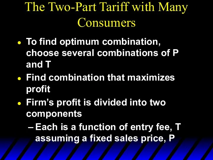
- 84. The Two-Part Tariff with Many Consumers To find optimum combination, choose several combinations of P and
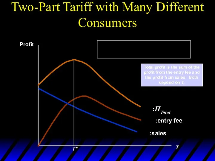
- 85. Two-Part Tariff with Many Different Consumers T Profit Total profit is the sum of the profit
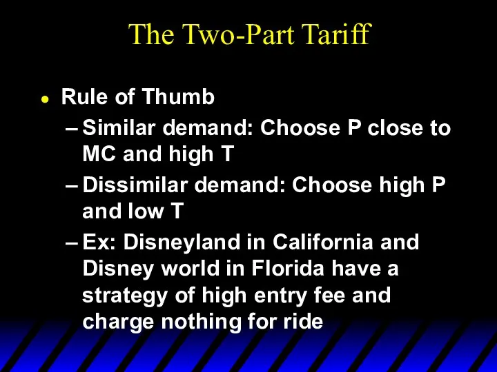
- 86. The Two-Part Tariff Rule of Thumb Similar demand: Choose P close to MC and high T
- 87. The Two-Part Tariff With a Twist Entry price (T) entitles the buyer to a certain number
- 88. Polaroid Cameras In 1971, Polaroid introduced the SX-70 camera Polaroid was able to use two-part tariff
- 89. Polaroid Cameras Buying camera is like entry fee Unlike an amusement park, for example, the marginal
- 90. Polaroid Cameras Analytical framework:
- 91. Polaroid Cameras In the end, the film prices were significantly above marginal cost There was considerable
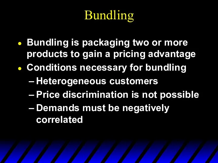
- 92. Bundling Bundling is packaging two or more products to gain a pricing advantage Conditions necessary for
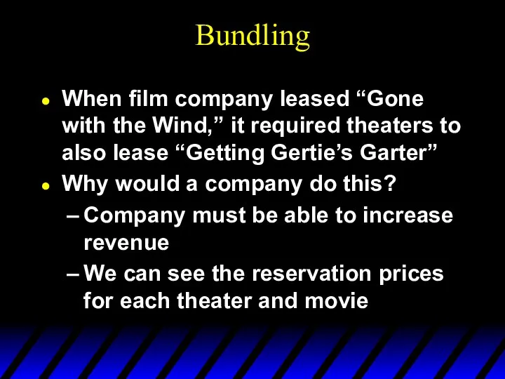
- 93. Bundling When film company leased “Gone with the Wind,” it required theaters to also lease “Getting
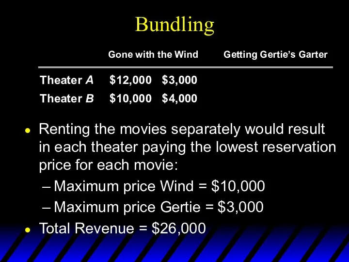
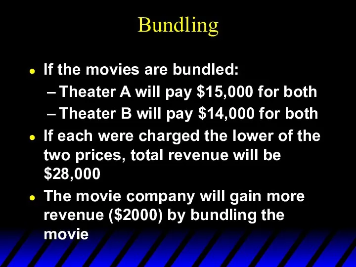
- 94. Bundling Renting the movies separately would result in each theater paying the lowest reservation price for
- 95. Bundling If the movies are bundled: Theater A will pay $15,000 for both Theater B will
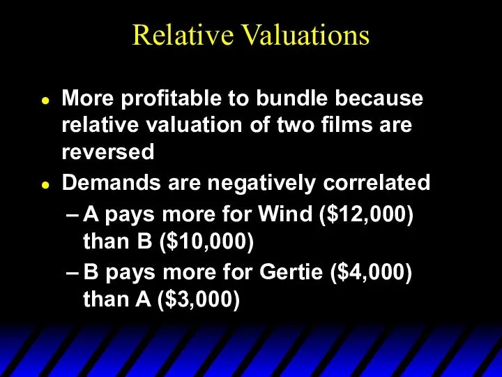
- 96. Relative Valuations More profitable to bundle because relative valuation of two films are reversed Demands are
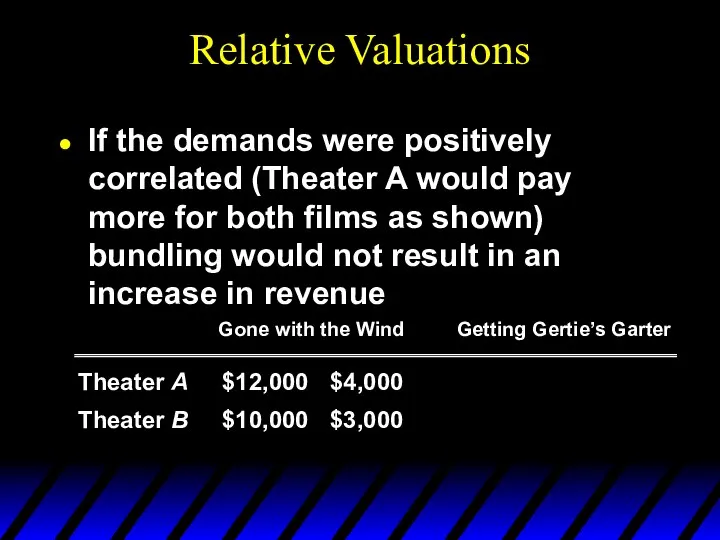
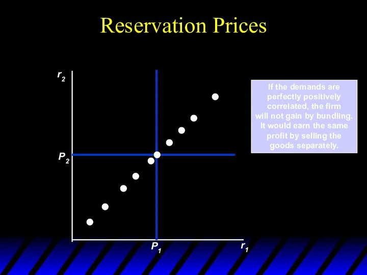
- 97. Relative Valuations If the demands were positively correlated (Theater A would pay more for both films
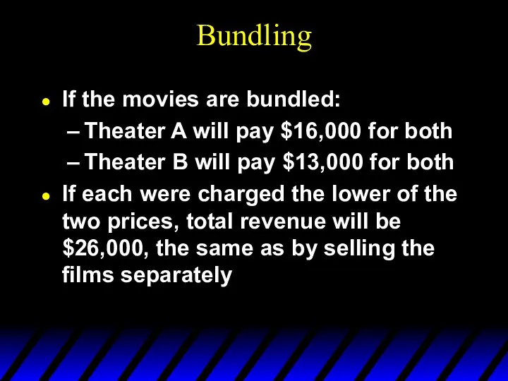
- 98. Bundling If the movies are bundled: Theater A will pay $16,000 for both Theater B will
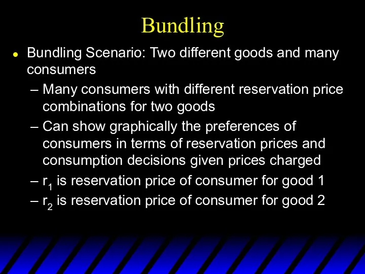
- 99. Bundling Bundling Scenario: Two different goods and many consumers Many consumers with different reservation price combinations
- 100. Reservation Prices r2 r1 For example, Consumer A is willing to pay up to $3.25 for
- 101. Consumption Decisions When Products are Sold Separately r2 r1 Consumers fall into four categories based on
- 102. Consumption Decisions When Products are Bundled r2 r1 Consumers buy the bundle when r1 + r2
- 103. Consumption Decisions When Products are Bundled The effectiveness of bundling depends upon the degree of negative
- 104. Reservation Prices If the demands are perfectly positively correlated, the firm will not gain by bundling.
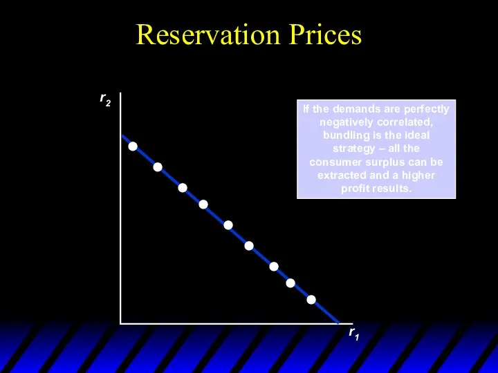
- 105. Reservation Prices r2 r1 If the demands are perfectly negatively correlated, bundling is the ideal strategy
- 106. Movie Example r2 r1 Bundling pays due to negative correlation. (Wind) (Gertie) 5,000 14,000 10,000 5,000
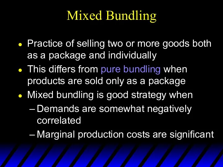
- 107. Mixed Bundling Practice of selling two or more goods both as a package and individually This
- 108. Mixed Versus Pure Bundling For each good, marginal production cost exceeds reservation price of one consumer.
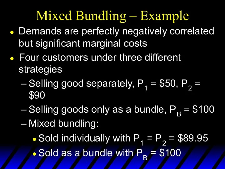
- 109. Mixed Bundling – Example Demands are perfectly negatively correlated but significant marginal costs Four customers under
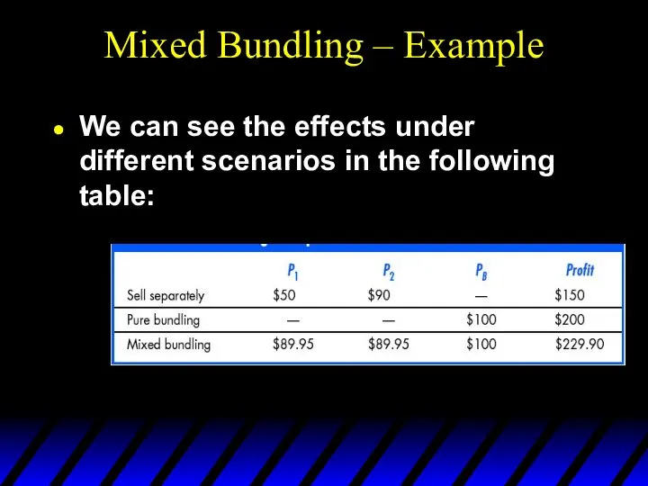
- 110. Mixed Bundling – Example We can see the effects under different scenarios in the following table:
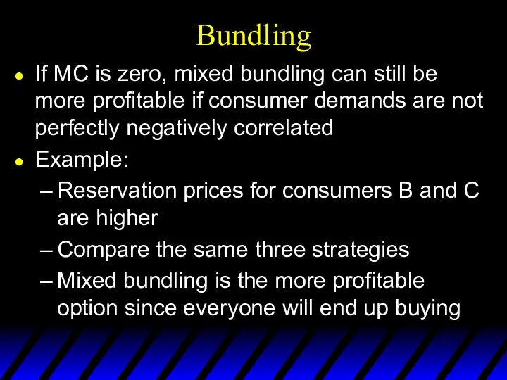
- 111. Bundling If MC is zero, mixed bundling can still be more profitable if consumer demands are
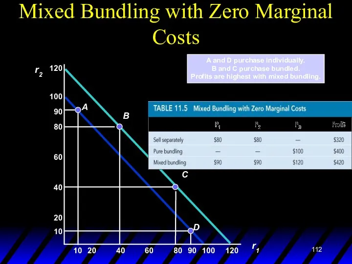
- 112. Mixed Bundling with Zero Marginal Costs A and D purchase individually. B and C purchase bundled.
- 113. Bundling in Practice Car purchasing Bundles of options such as electric locks with air conditioning Vacation
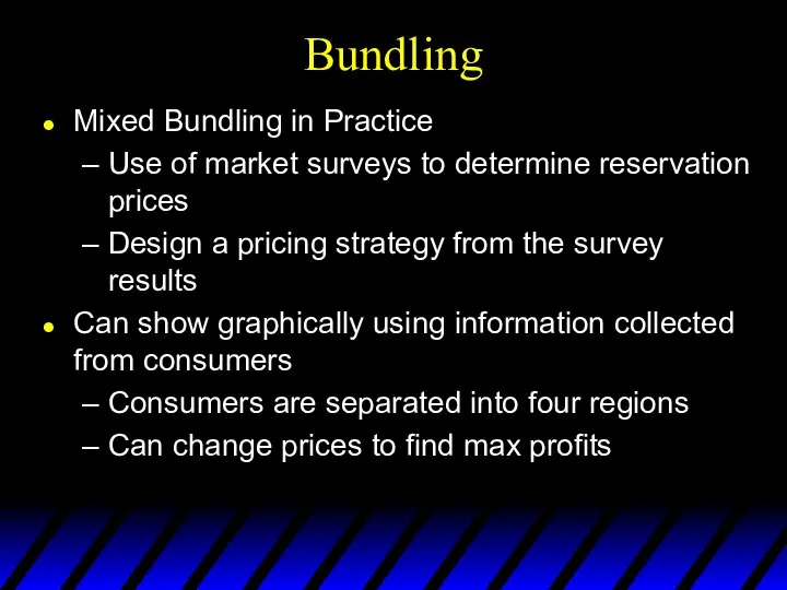
- 114. Bundling Mixed Bundling in Practice Use of market surveys to determine reservation prices Design a pricing
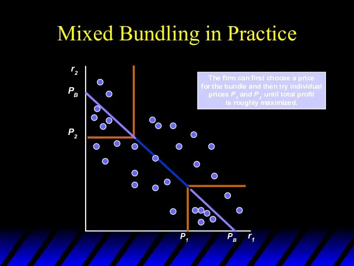
- 115. Mixed Bundling in Practice r2 r1 The firm can first choose a price for the bundle
- 116. A Restaurant’s Pricing Problem
- 117. Tying The practice of requiring a customer to purchase one good in order to purchase another
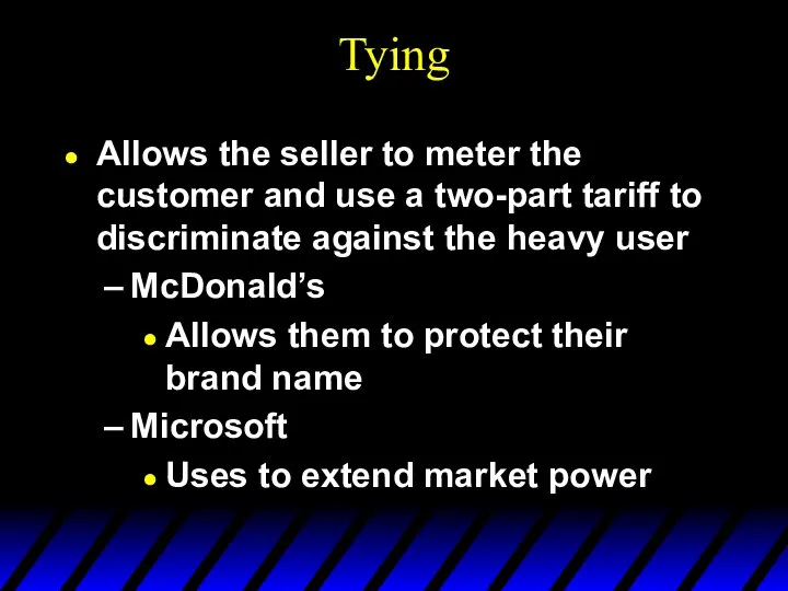
- 118. Tying Allows the seller to meter the customer and use a two-part tariff to discriminate against
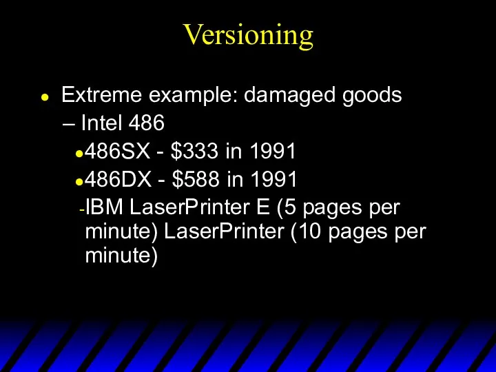
- 119. Versioning Extreme example: damaged goods Intel 486 486SX - $333 in 1991 486DX - $588 in
- 120. Durable-goods pricing Waiting for the price cut. Non-price discrimination seems to increase profits Possible solutions: lowest
- 121. Advertising Firms with market power have to decide how much to advertise We can show how
- 122. Advertising Assumptions Firm sets only one price for product Firm knows quantity demanded depends on price
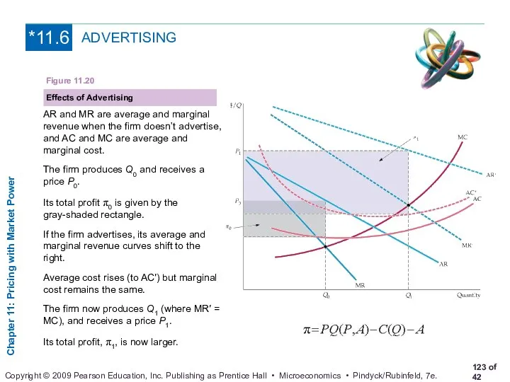
- 123. ADVERTISING Effects of Advertising Figure 11.20 AR and MR are average and marginal revenue when the
- 124. The price P and advertising expenditure A to maximize profit, is given by: The firm should
- 125. First, rewrite equation (11.3) as follows: Now multiply both sides of this equation by A/PQ, the
- 126. Advertising A Rule of Thumb for Advertising To maximize profit, the firm’s advertising-to-sales ratio should be
- 127. Advertising An Example R(Q) = $1 million/yr $10,000 budget for A (advertising--1% of revenues) EA =
- 128. Advertising The firm in our example should increase advertising A/PQ = -(2/-.4) = 5% Increase budget
- 130. Скачать презентацию
A Scotsman phones a dentist to inquire about the cost for
A Scotsman phones a dentist to inquire about the cost for

— "I can't guarantee their professionalism and it'll be painful. But
— "I can't guarantee their professionalism and it'll be painful. But
How Should a Monopoly Price?
So far a monopoly has been thought
How Should a Monopoly Price?
So far a monopoly has been thought
Capturing Consumer Surplus
All pricing strategies we will examine are means of
Capturing Consumer Surplus
All pricing strategies we will examine are means of
Capturing Consumer Surplus
Quantity
$/Q
The firm would like to charge higher price to
Capturing Consumer Surplus
Quantity
$/Q
The firm would like to charge higher price to

Capturing Consumer Surplus
Price discrimination is the practice of charging different prices
Capturing Consumer Surplus
Price discrimination is the practice of charging different prices
Price discrimination
Price discrimination requires the absence of resale
Price discrimination
Price discrimination requires the absence of resale
Types of Price Discrimination
1st-degree: Each output unit is sold at a
Types of Price Discrimination
1st-degree: Each output unit is sold at a
Types of Price Discrimination
3rd-degree: Price paid by buyers in a given
Types of Price Discrimination
3rd-degree: Price paid by buyers in a given
First-degree Price Discrimination
Each output unit is sold at a different price.
First-degree Price Discrimination
Each output unit is sold at a different price.
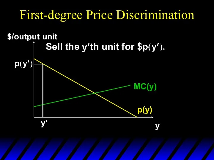
First-degree Price Discrimination
p(y)
y
$/output unit
MC(y)
Sell the th unit for $
First-degree Price Discrimination
p(y)
y
$/output unit
MC(y)
Sell the th unit for $
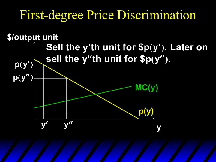
First-degree Price Discrimination
p(y)
y
$/output unit
MC(y)
Sell the th unit for $ Later on
sell
First-degree Price Discrimination
p(y)
y
$/output unit
MC(y)
Sell the th unit for $ Later on sell
First-degree Price Discrimination
p(y)
y
$/output unit
MC(y)
Sell the th unit for $ Later on
sell
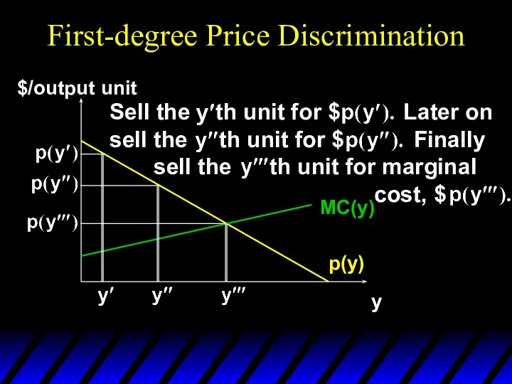
First-degree Price Discrimination
p(y)
y
$/output unit
MC(y)
Sell the th unit for $ Later on sell
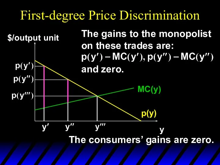
First-degree Price Discrimination
p(y)
y
$/output unit
MC(y)
The gains to the monopolist
on these trades are:
and
First-degree Price Discrimination
p(y)
y
$/output unit
MC(y)
The gains to the monopolist on these trades are: and
First-degree Price Discrimination
p(y)
y
$/output unit
MC(y)
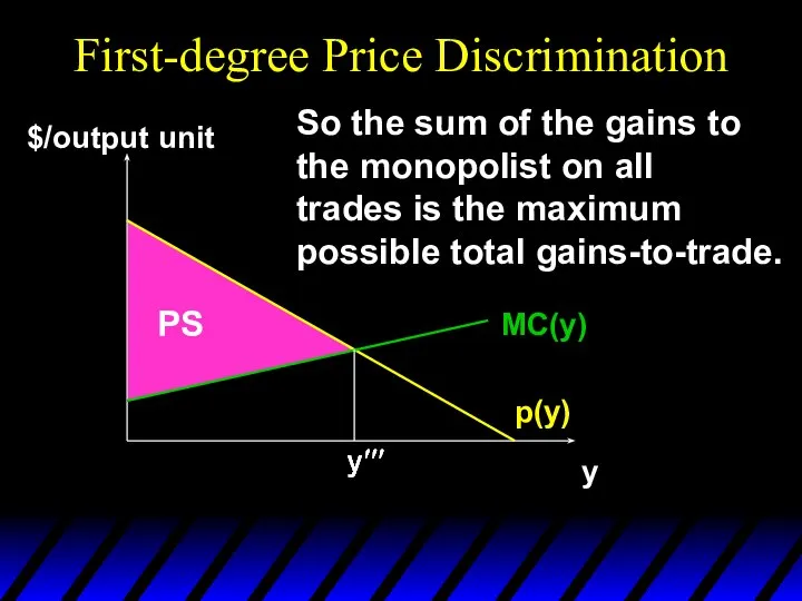
So the sum of the gains to
the monopolist
First-degree Price Discrimination
p(y)
y
$/output unit
MC(y)
So the sum of the gains to the monopolist
First-degree Price Discrimination
p(y)
y
$/output unit
MC(y)
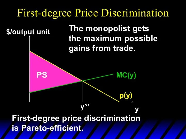
The monopolist gets
the maximum possible
gains from
First-degree Price Discrimination
p(y)
y
$/output unit
MC(y)
The monopolist gets
the maximum possible
gains from

Fig. 25.2
Fig. 25.2
First-degree Price Discrimination
First-degree price discrimination gives a monopolist all of the
First-degree Price Discrimination
First-degree price discrimination gives a monopolist all of the
First-Degree Price Discrimination
In practice, perfect price discrimination is almost never possible
Impractical
First-Degree Price Discrimination
In practice, perfect price discrimination is almost never possible
Impractical
First-Degree Price Discrimination
Examples of imperfect price discrimination where the seller has
First-Degree Price Discrimination
Examples of imperfect price discrimination where the seller has
Second-Degree Price Discrimination
In some markets, consumers purchase many units of a
Second-Degree Price Discrimination
In some markets, consumers purchase many units of a
Second-Degree Price Discrimination
Quantity discounts are an example of second-degree price discrimination
Ex:
Second-Degree Price Discrimination
Quantity discounts are an example of second-degree price discrimination
Ex:
Second-Degree Price Discrimination
$/Q
Without discrimination:
P = P0 and Q = Q0.
Second-Degree Price Discrimination
$/Q
Without discrimination: P = P0 and Q = Q0.
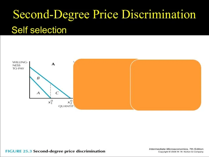
Fig. 25.3
Second-Degree Price Discrimination
Self selection
Fig. 25.3
Second-Degree Price Discrimination
Self selection
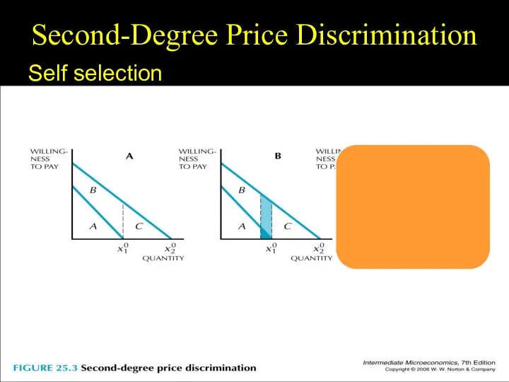
Fig. 25.3
Second-Degree Price Discrimination
Self selection
Fig. 25.3
Second-Degree Price Discrimination
Self selection
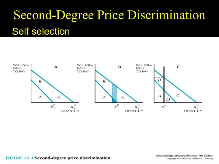
Fig. 25.3
Second-Degree Price Discrimination
Self selection
Fig. 25.3
Second-Degree Price Discrimination
Self selection
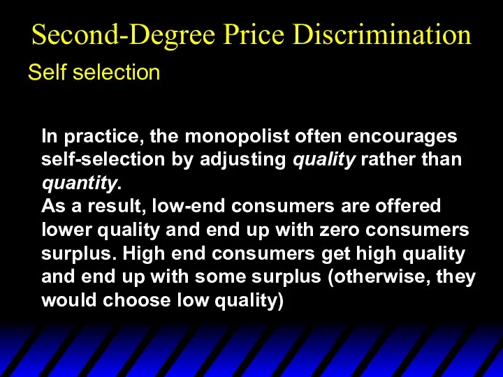
Fig. 25.3
Second-Degree Price Discrimination
Self selection
In practice, the monopolist often encourages self-selection
Fig. 25.3
Second-Degree Price Discrimination
Self selection
In practice, the monopolist often encourages self-selection
Third-degree Price Discrimination
Price paid by buyers in a given group is
Third-degree Price Discrimination
Price paid by buyers in a given group is
Third-degree Price Discrimination
A monopolist manipulates market price by altering the quantity
Third-degree Price Discrimination
A monopolist manipulates market price by altering the quantity
PRICE DISCRIMINATION
Third-Degree Price Discrimination
● third-degree price discrimination Practice of dividing consumers into
PRICE DISCRIMINATION
Third-Degree Price Discrimination
● third-degree price discrimination Practice of dividing consumers into
PRICE DISCRIMINATION
Third-Degree Price Discrimination
Creating Consumer Groups
Determining Relative Prices
PRICE DISCRIMINATION
Third-Degree Price Discrimination
Creating Consumer Groups
Determining Relative Prices
PRICE DISCRIMINATION
Third-Degree Price Discrimination
Third-Degree Price Discrimination
Figure 11.5
Consumers are divided into two
PRICE DISCRIMINATION
Third-Degree Price Discrimination
Third-Degree Price Discrimination
Figure 11.5
Consumers are divided into two
Third-degree Price Discrimination
MR1(y1)
MR2(y2)
y1
y2
y1*
y2*
p1(y1*)
p2(y2*)
MC
MC
p1(y1)
p2(y2)
Market 1
Market 2
MR1(y1*) = MR2(y2*) = MC
Third-degree Price Discrimination
MR1(y1)
MR2(y2)
y1
y2
y1*
y2*
p1(y1*)
p2(y2*)
MC
MC
p1(y1)
p2(y2)
Market 1
Market 2
MR1(y1*) = MR2(y2*) = MC

Third-degree Price Discrimination
MR1(y1)
MR2(y2)
y1
y2
y1*
y2*
p1(y1*)
p2(y2*)
MC
MC
p1(y1)
p2(y2)
Market 1
Market 2
MR1(y1*) = MR2(y2*) = MC and p1(y1*)
Third-degree Price Discrimination
MR1(y1)
MR2(y2)
y1
y2
y1*
y2*
p1(y1*)
p2(y2*)
MC
MC
p1(y1)
p2(y2)
Market 1
Market 2
MR1(y1*) = MR2(y2*) = MC and p1(y1*)

Third-degree Price Discrimination
In which market will the monopolist cause the higher
Third-degree Price Discrimination
In which market will the monopolist cause the higher
Third-degree Price Discrimination
In which market will the monopolist cause the higher
Third-degree Price Discrimination
In which market will the monopolist cause the higher
Third-degree Price Discrimination
In which market will the monopolist cause the higher
Third-degree Price Discrimination
In which market will the monopolist cause the higher
Third-degree Price Discrimination
So
Third-degree Price Discrimination
So
Third-degree Price Discrimination
So
Therefore, if and only if
Third-degree Price Discrimination
So
Therefore, if and only if
Third-degree Price Discrimination
So
Therefore, if and only if
Third-degree Price Discrimination
So
Therefore, if and only if

Third-degree Price Discrimination
So
Therefore, if and only if
The monopolist sets the higher
Third-degree Price Discrimination
So
Therefore, if and only if
The monopolist sets the higher
No Sales to Smaller Market
Even if third-degree price discrimination is possible,
No Sales to Smaller Market
Even if third-degree price discrimination is possible,
No Sales to Smaller Market
Quantity
$/Q
Group one, with
demand D1, is not
No Sales to Smaller Market
Quantity
$/Q
Group one, with
demand D1, is not
The Economics of Coupons
and Rebates
Those consumers who are more price
The Economics of Coupons
and Rebates
Those consumers who are more price
The Economics of Coupons
and Rebates
About 20 – 30% of consumers
The Economics of Coupons
and Rebates
About 20 – 30% of consumers
Price Elasticities of Demand: Users vs. Nonusers of Coupons
Price Elasticities of Demand: Users vs. Nonusers of Coupons
Airline Fares
Differences in elasticities imply that some customers will pay a
Airline Fares
Differences in elasticities imply that some customers will pay a

Elasticities of Demand for
Air Travel
Elasticities of Demand for
Air Travel
Airline Fares
There are multiple fares for every route flown by airlines
They
Airline Fares
There are multiple fares for every route flown by airlines
They
Other Types of Price Discrimination
Intertemporal Price Discrimination
Practice of separating consumers with
Other Types of Price Discrimination
Intertemporal Price Discrimination
Practice of separating consumers with

Intertemporal Price Discrimination
Once this market has yielded a maximum profit, firms
Intertemporal Price Discrimination
Once this market has yielded a maximum profit, firms
Intertemporal Price Discrimination
Quantity
$/Q
Over time, demand becomes
more elastic and price
is reduced
Intertemporal Price Discrimination
Quantity
$/Q
Over time, demand becomes
more elastic and price
is reduced
Other Types of Price Discrimination
Peak-Load Pricing
Practice of charging higher prices during
Other Types of Price Discrimination
Peak-Load Pricing
Practice of charging higher prices during

Peak-Load Pricing
Objective is to increase efficiency by charging customers close to
Peak-Load Pricing
Objective is to increase efficiency by charging customers close to
Peak-Load Pricing
With third-degree price discrimination, the MR for all markets was
Peak-Load Pricing
With third-degree price discrimination, the MR for all markets was
Peak-Load Pricing
Quantity
$/Q
MR=MC for each group. Group 1 has higher demand during
Peak-Load Pricing
Quantity
$/Q
MR=MC for each group. Group 1 has higher demand during
How to Price a Best-Selling Novel
How would you arrive at the
How to Price a Best-Selling Novel
How would you arrive at the
How to Price a Best-Selling Novel
Company must divide consumers into two
How to Price a Best-Selling Novel
Company must divide consumers into two
How to Price a Best-Selling Novel
Publishers must use estimates of past
How to Price a Best-Selling Novel
Publishers must use estimates of past
Two-Part Tariffs
A two-part tariff is a lump-sum fee, p1, plus a
Two-Part Tariffs
A two-part tariff is a lump-sum fee, p1, plus a
Two-Part Tariffs
Should a monopolist prefer a two-part tariff to uniform pricing,
Two-Part Tariffs
Should a monopolist prefer a two-part tariff to uniform pricing,
Two-Part Tariffs
p1 + p2x
Q: What is the largest that p1
Two-Part Tariffs
p1 + p2x
Q: What is the largest that p1
Two-Part Tariffs
p1 + p2x
Q: What is the largest that p1
Two-Part Tariffs
p1 + p2x
Q: What is the largest that p1
Two-Part Tariffs
p(y)
y
$/output unit
MC(y)
Should the monopolist
set p2 above MC?
Two-Part Tariffs
p(y)
y
$/output unit
MC(y)
Should the monopolist
set p2 above MC?
Two-Part Tariffs
p(y)
y
$/output unit
CS
Should the monopolist
set p2 above MC?
p1 = CS.
MC(y)
Two-Part Tariffs
p(y)
y
$/output unit
CS
Should the monopolist
set p2 above MC?
p1 = CS.
MC(y)
Two-Part Tariffs
p(y)
y
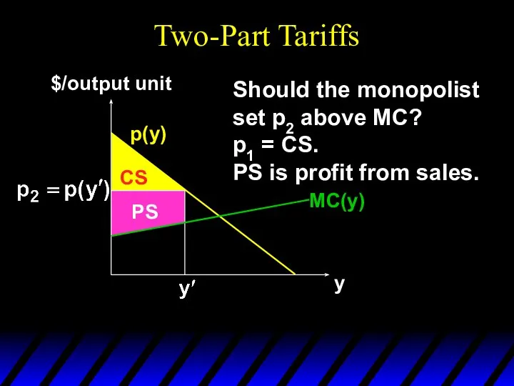
$/output unit
CS
Should the monopolist
set p2 above MC?
p1 = CS.
PS is
Two-Part Tariffs
p(y)
y
$/output unit
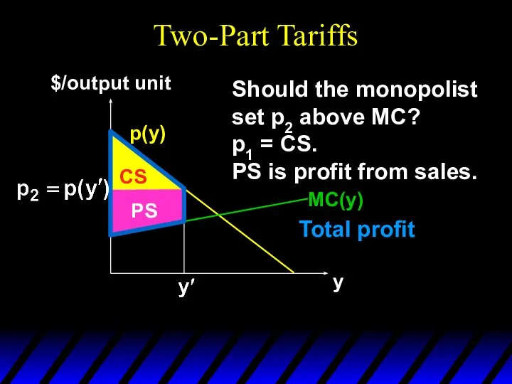
CS
Should the monopolist set p2 above MC? p1 = CS. PS is
Two-Part Tariffs
p(y)
y
$/output unit
CS
Should the monopolist
set p2 above MC?
p1 = CS.
PS is
Two-Part Tariffs
p(y)
y
$/output unit
CS
Should the monopolist set p2 above MC? p1 = CS. PS is
Two-Part Tariffs
p(y)
y
$/output unit
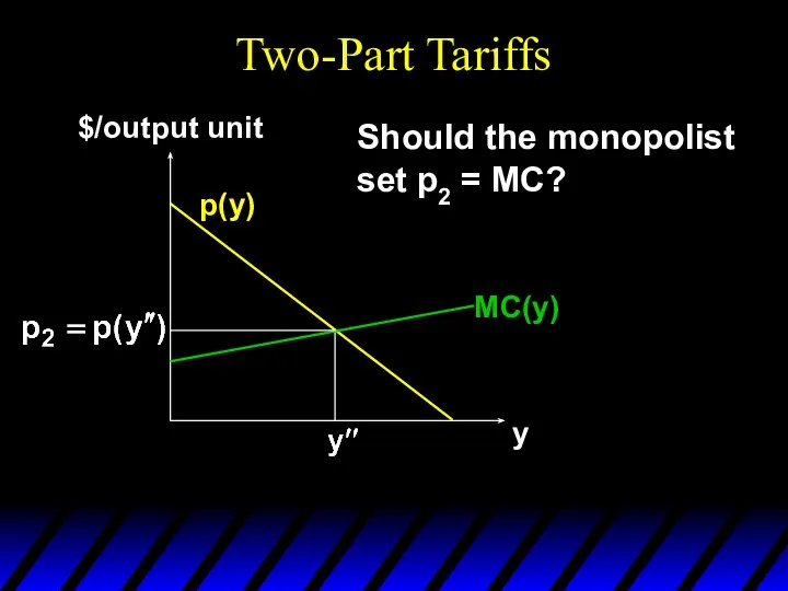
Should the monopolist
set p2 = MC?
MC(y)
Two-Part Tariffs
p(y)
y
$/output unit
Should the monopolist
set p2 = MC?
MC(y)

Two-Part Tariffs
p(y)
y
$/output unit
Should the monopolist
set p2 = MC?
p1 = CS.
CS
MC(y)
Two-Part Tariffs
p(y)
y
$/output unit
Should the monopolist
set p2 = MC?
p1 = CS.
CS
MC(y)
Two-Part Tariffs
p(y)
y
$/output unit
Should the monopolist
set p2 = MC?
p1 = CS.
PS is
Two-Part Tariffs
p(y)
y
$/output unit
Should the monopolist set p2 = MC? p1 = CS. PS is
Two-Part Tariffs
p(y)
y
$/output unit
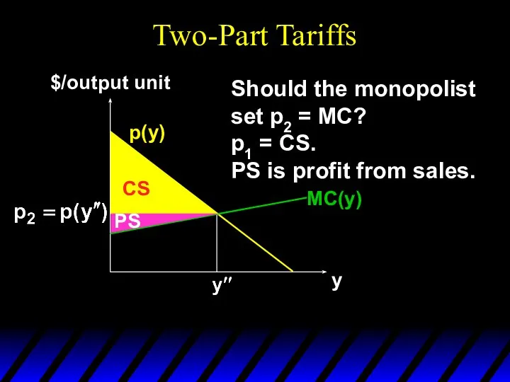
Should the monopolist
set p2 = MC?
p1 = CS.
PS is
Two-Part Tariffs
p(y)
y
$/output unit
Should the monopolist set p2 = MC? p1 = CS. PS is
Two-Part Tariffs
p(y)
y
$/output unit
Should the monopolist
set p2 = MC?
p1 = CS.
PS is
Two-Part Tariffs
p(y)
y
$/output unit
Should the monopolist set p2 = MC? p1 = CS. PS is
Two-Part Tariffs
p(y)
y
$/output unit
Should the monopolist
set p2 = MC?
p1 = CS.
PS is
Two-Part Tariffs
p(y)
y
$/output unit
Should the monopolist set p2 = MC? p1 = CS. PS is

Two-Part Tariffs
The monopolist maximizes its profit when using a two-part tariff
Two-Part Tariffs
The monopolist maximizes its profit when using a two-part tariff
Two-Part Tariffs
A profit-maximizing two-part tariff gives an efficient market outcome in
Two-Part Tariffs
A profit-maximizing two-part tariff gives an efficient market outcome in
The Two-Part Tariff
Form of pricing in which consumers are charged both
The Two-Part Tariff
Form of pricing in which consumers are charged both
The Two-Part Tariff
Pricing decision is setting the entry fee (T) and
The Two-Part Tariff
Pricing decision is setting the entry fee (T) and
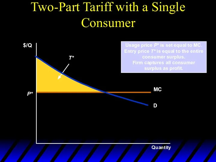
Usage price P* is set equal to MC.
Entry price T*
Usage price P* is set equal to MC.
Entry price T*
Two-Part Tariff with Two Consumers
Two consumers, but firm can only set
Two-Part Tariff with Two Consumers
Two consumers, but firm can only set

The price, P*, will be
greater than MC. Set T*
at
The price, P*, will be
greater than MC. Set T*
at
Two-Part Tariff with Two Consumers
Firm should set usage fee above MC
Set
Two-Part Tariff with Two Consumers
Firm should set usage fee above MC
Set

The Two-Part Tariff with Many Consumers
No exact way to determine P*
The Two-Part Tariff with Many Consumers
No exact way to determine P*
The Two-Part Tariff with Many Consumers
To find optimum combination, choose several
The Two-Part Tariff with Many Consumers
To find optimum combination, choose several
Two-Part Tariff with Many Different Consumers
T
Profit
Total profit is the sum of
Two-Part Tariff with Many Different Consumers
T
Profit
Total profit is the sum of
The Two-Part Tariff
Rule of Thumb
Similar demand: Choose P close to MC
The Two-Part Tariff
Rule of Thumb
Similar demand: Choose P close to MC
The Two-Part Tariff With a Twist
Entry price (T) entitles the buyer
The Two-Part Tariff With a Twist
Entry price (T) entitles the buyer
Polaroid Cameras
In 1971, Polaroid introduced the SX-70 camera
Polaroid was able to
Polaroid Cameras
In 1971, Polaroid introduced the SX-70 camera
Polaroid was able to
Polaroid Cameras
Buying camera is like entry fee
Unlike an amusement park, for
Polaroid Cameras
Buying camera is like entry fee
Unlike an amusement park, for
Polaroid Cameras
Analytical framework:
Polaroid Cameras
Analytical framework:
Polaroid Cameras
In the end, the film prices were significantly above marginal
Polaroid Cameras
In the end, the film prices were significantly above marginal
Bundling
Bundling is packaging two or more products to gain a pricing
Bundling
Bundling is packaging two or more products to gain a pricing
Bundling
When film company leased “Gone with the Wind,” it required theaters
Bundling
When film company leased “Gone with the Wind,” it required theaters
Bundling
Renting the movies separately would result in each theater paying the
Bundling
Renting the movies separately would result in each theater paying the
Bundling
If the movies are bundled:
Theater A will pay $15,000 for both
Theater
Bundling
If the movies are bundled:
Theater A will pay $15,000 for both
Theater
Relative Valuations
More profitable to bundle because relative valuation of two films
Relative Valuations
More profitable to bundle because relative valuation of two films
Relative Valuations
If the demands were positively correlated (Theater A would pay
Relative Valuations
If the demands were positively correlated (Theater A would pay
Bundling
If the movies are bundled:
Theater A will pay $16,000 for both
Theater
Bundling
If the movies are bundled:
Theater A will pay $16,000 for both
Theater
Bundling
Bundling Scenario: Two different goods and many consumers
Many consumers with different
Bundling
Bundling Scenario: Two different goods and many consumers
Many consumers with different

Reservation Prices
r2
r1
For example, Consumer A is willing to pay up
Reservation Prices
r2
r1
For example, Consumer A is willing to pay up
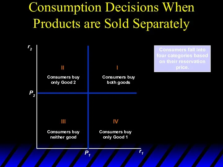
Consumption Decisions When
Products are Sold Separately
r2
r1
Consumers fall into
four categories based
on their
Consumption Decisions When
Products are Sold Separately
r2
r1
Consumers fall into
four categories based
on their
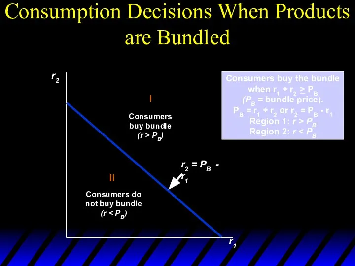
Consumption Decisions When Products are Bundled
r2
r1
Consumers buy the bundle
when r1 +
Consumption Decisions When Products are Bundled
r2
r1
Consumers buy the bundle
when r1 +
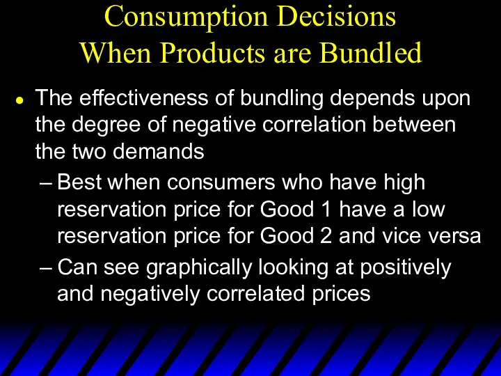
Consumption Decisions
When Products are Bundled
The effectiveness of bundling depends upon the
Consumption Decisions
When Products are Bundled
The effectiveness of bundling depends upon the
Reservation Prices
If the demands are
perfectly positively
correlated, the firm
will not gain
Reservation Prices
If the demands are
perfectly positively
correlated, the firm
will not gain
Reservation Prices
r2
r1
If the demands are perfectly negatively correlated, bundling is the
Reservation Prices
r2
r1
If the demands are perfectly negatively correlated, bundling is the
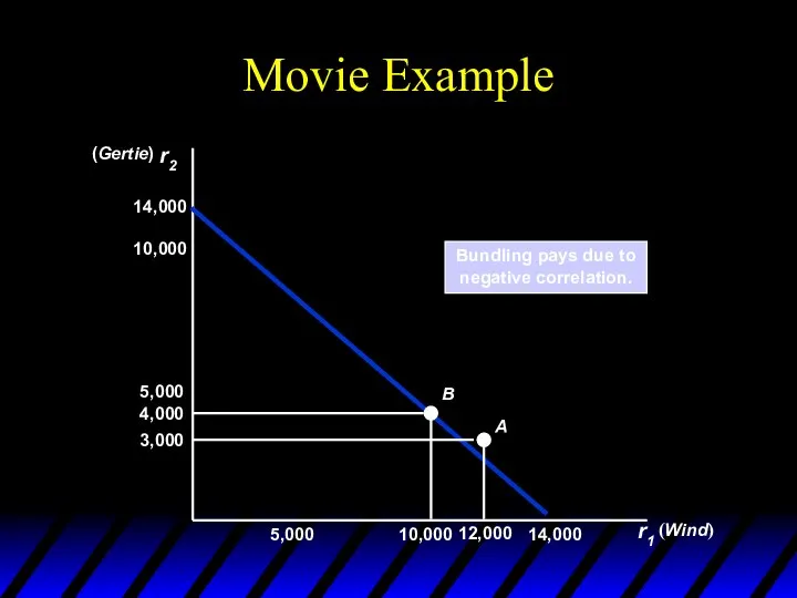
Movie Example
r2
r1
Bundling pays due to
negative correlation.
(Wind)
(Gertie)
5,000
14,000
10,000
5,000
10,000
14,000
Movie Example
r2
r1
Bundling pays due to
negative correlation.
(Wind)
(Gertie)
5,000
14,000
10,000
5,000
10,000
14,000
Mixed Bundling
Practice of selling two or more goods both as a
Mixed Bundling
Practice of selling two or more goods both as a

Mixed Versus Pure Bundling
For each good, marginal production cost exceeds reservation
Mixed Versus Pure Bundling
For each good, marginal production cost exceeds reservation
Mixed Bundling – Example
Demands are perfectly negatively correlated but significant marginal
Mixed Bundling – Example
Demands are perfectly negatively correlated but significant marginal
Mixed Bundling – Example
We can see the effects under different scenarios
Mixed Bundling – Example
We can see the effects under different scenarios
Bundling
If MC is zero, mixed bundling can still be more profitable
Bundling
If MC is zero, mixed bundling can still be more profitable
Mixed Bundling with Zero Marginal Costs
A and D purchase individually.
B and
Mixed Bundling with Zero Marginal Costs
A and D purchase individually.
B and

Bundling in Practice
Car purchasing
Bundles of options such as electric locks with
Bundling in Practice
Car purchasing
Bundles of options such as electric locks with
Bundling
Mixed Bundling in Practice
Use of market surveys to determine reservation prices
Design
Bundling
Mixed Bundling in Practice
Use of market surveys to determine reservation prices
Design
Mixed Bundling in Practice
r2
r1
The firm can first choose a price
for the
Mixed Bundling in Practice
r2
r1
The firm can first choose a price
for the

A Restaurant’s Pricing Problem
A Restaurant’s Pricing Problem

Tying
The practice of requiring a customer to purchase one good in
Tying
The practice of requiring a customer to purchase one good in
Tying
Allows the seller to meter the customer and use a two-part
Tying
Allows the seller to meter the customer and use a two-part
Versioning
Extreme example: damaged goods
Intel 486
486SX - $333 in 1991
486DX -
Versioning
Extreme example: damaged goods
Intel 486
486SX - $333 in 1991
486DX -

Durable-goods pricing
Waiting for the price cut.
Non-price discrimination seems to increase profits
Possible
Durable-goods pricing
Waiting for the price cut.
Non-price discrimination seems to increase profits
Possible
Advertising
Firms with market power have to decide how much to advertise
We
Advertising
Firms with market power have to decide how much to advertise
We
Advertising
Assumptions
Firm sets only one price for product
Firm knows quantity demanded depends
Advertising
Assumptions
Firm sets only one price for product
Firm knows quantity demanded depends
ADVERTISING
Effects of Advertising
Figure 11.20
AR and MR are average and marginal revenue
ADVERTISING
Effects of Advertising
Figure 11.20
AR and MR are average and marginal revenue
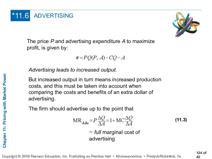
The price P and advertising expenditure A to maximize profit, is
The price P and advertising expenditure A to maximize profit, is
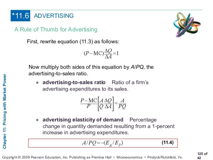
First, rewrite equation (11.3) as follows:
Now multiply both sides of this
First, rewrite equation (11.3) as follows:
Now multiply both sides of this

Advertising
A Rule of Thumb for Advertising
To maximize profit, the firm’s advertising-to-sales
Advertising
A Rule of Thumb for Advertising
To maximize profit, the firm’s advertising-to-sales
Advertising
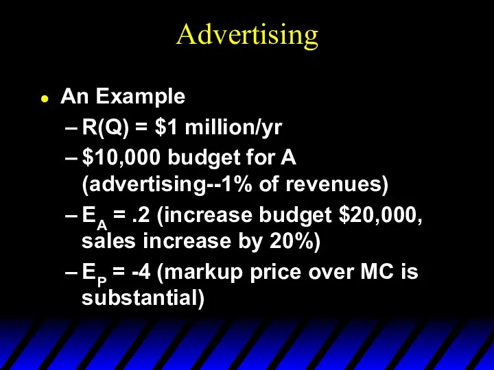
An Example
R(Q) = $1 million/yr
$10,000 budget for A (advertising--1% of revenues)
EA
Advertising
An Example
R(Q) = $1 million/yr
$10,000 budget for A (advertising--1% of revenues)
EA
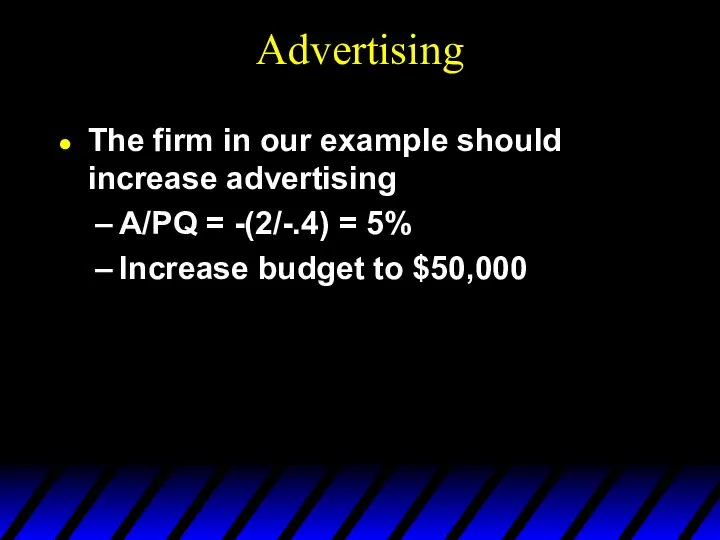
Advertising
The firm in our example should increase advertising
A/PQ = -(2/-.4) =
Advertising
The firm in our example should increase advertising
A/PQ = -(2/-.4) =
 Презентация Издержки производства и прибыль
 Стратегическое финансирование. Построение график безубыточности предприятия
 Цінність грошей в часі. (Тема 5)
 Фінансово-економічні результати діяльності підприємства СФГ Буштрука Є.В, та напрямки їх поліпшення
 Экономический рост. Цикличность экономического развития
 Раціональна поведінка споживача та її аналіз
 Предпринимательство и модели бизнеса. Модели бизнеса
 Внешнеторговые отношения
 Экономическая теория. Формы общественного хозяйства
 Доходы бюджета РФ (данные за 2013 год) и роль ФТС. Подготовили: Калинина Екатерина Жуков Никита
 Региональные интеграционные блоки Японии
 Презентация Сущность налогов и налогообложения
 Қазақстанның шет елдермен қарым-қатынасы және дипломатиясы
 Виды ценовой дискриминации
 Основные фонды предприятия
 Коммунизм – сила, капитализм – могила. Тренинг
 Україна - Швеція
 Экономика, как наука и хозяйство
 Экономический анализ, как метод познания и обоснования экономических решений
 Аттестационная работа. Методические указания по выполнению проекта на занятиях экономики
 Классическая школа
 Цикличность экономического развития как закономерность макроэкономики. Лекция 9
 Экономика образования. Сущность материально-технической базы и состав фондов образования
 Введение в макроэкономику
 Предложение по формированию концепции создания фонда «Труда и социальной поддержки»
 Государство и экономика
 Теория фирмы
 Проект- огород «Успешная ферма»