- Aerodynamics I

Содержание
- 2. Useful Info
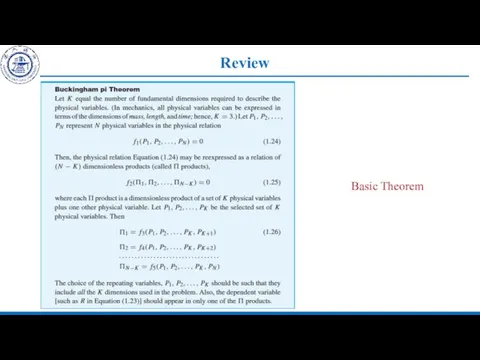
- 3. Review The Principle of Dimensional Homogeneity (PDH)——a rule which is almost a self-evident axiom in physics
- 4. Review Basic Theorem
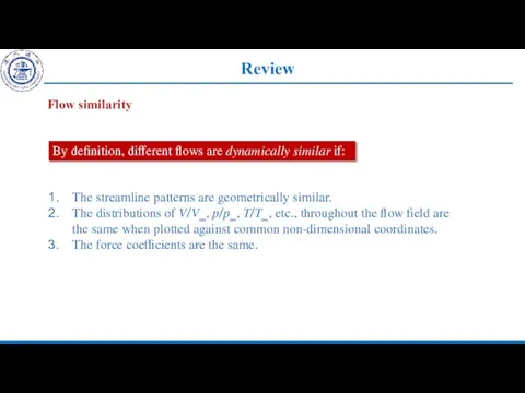
- 5. Review Flow similarity By definition, different flows are dynamically similar if: The streamline patterns are geometrically
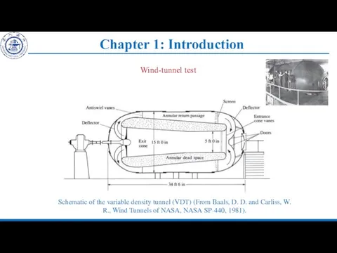
- 6. Chapter 1: Introduction Schematic of the variable density tunnel (VDT) (From Baals, D. D. and Carliss,
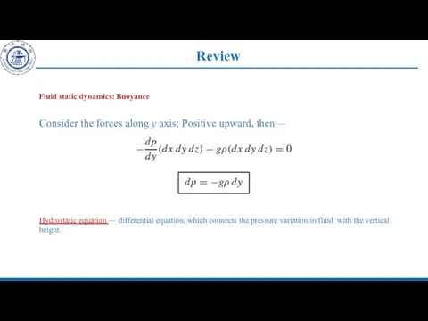
- 7. Review Fluid static dynamics: Buoyance Consider the forces along y axis: Positive upward, then— Hydrostatic equation
- 8. Review Type of flow Continuum flow If the orders of magnitude of λ is smaller than
- 9. Review Inviscid flow versus Viscous flow Viscous flow: This transport on a molecular scale gives rise
- 10. Course Diagram
- 11. Chapter 1 Learning Targets
- 12. Chapter 1: Introduction 1.11 Viscous flow: Brief introduction on boundary layer At any point in flow
- 13. Chapter 1: Introduction In 1904, Prandtl put forward the concept of boundary layer: boundary layer—the region
- 14. Chapter 1: Introduction Question: Why are the gradients so large inside the layer? Inviscid, no friction,
- 15. Chapter 1: Introduction Note: the above two are reasonable for the layer attached on the surface
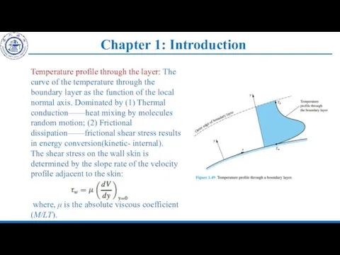
- 16. Chapter 1: Introduction Temperature profile through the layer: The curve of the temperature through the boundary
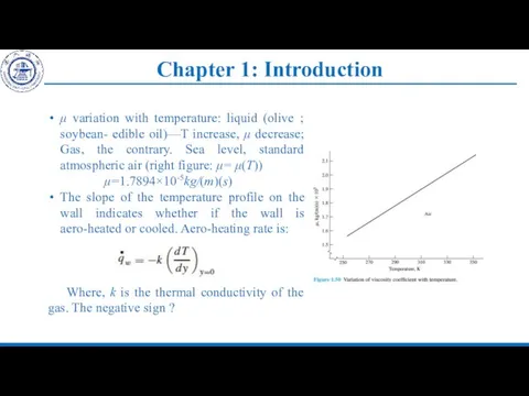
- 17. Chapter 1: Introduction μ variation with temperature: liquid (olive ; soybean- edible oil)—T increase, μ decrease;
- 18. Chapter 1: Introduction At standard sea level temperature: k=2.53×10⁻²J/(m)(s)(K) Proportional to the viscous coefficient essentially, i.e
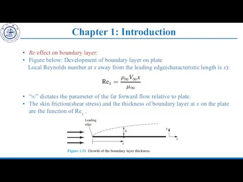
- 19. Chapter 1: Introduction Re effect on boundary layer: Figure below: Development of boundary layer on plate
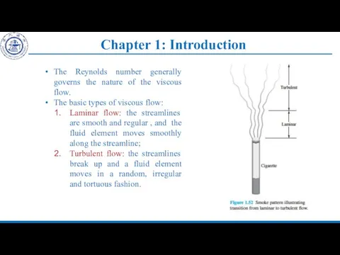
- 20. Chapter 1: Introduction The Reynolds number generally governs the nature of the viscous flow. The basic
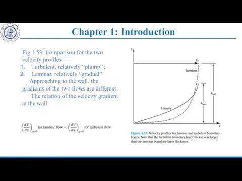
- 21. Chapter 1: Introduction Fig.1.53: Comparison for the two velocity profiles—— Turbulent, relatively “plump”; Laminar, relatively “gradual”.
- 22. Chapter 1: Introduction By Eq.1.59: (τw)laminer The important fact: The shear stress of laminar flow is
- 23. Chapter 1: Introduction Homework: 1.11, 1.12 Questions for thinking: 1. After released, the hydrogen ball will
- 24. Chapter 1: Introduction 1.12 Applied aerodynamics: Aerodynamic coefficients—— Magnitudes and variations Applied aerodynamics: For the practical
- 25. Chapter 1: Introduction Lift, Drag and moment coefficient are the most frequently used technical terms in
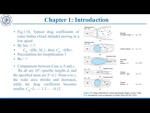
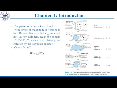
- 26. Chapter 1: Introduction Fig.1.54, Typical drag coefficients of some bodies (fixed attitude) moving in a low
- 27. Chapter 1: Introduction Comparisons between Case b and d : One order of magnitude difference in
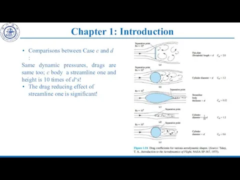
- 28. Chapter 1: Introduction Comparisons between Case c and d : Same dynamic pressures, drags are same
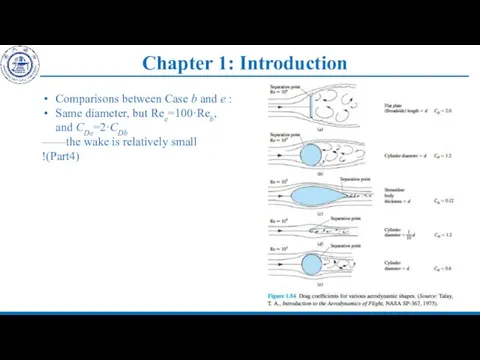
- 29. Chapter 1: Introduction Comparisons between Case b and e : Same diameter, but Ree=100·Reb, and CDe=2·CDb
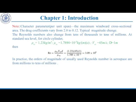
- 30. Chapter 1: Introduction Note:Character parameter(per unit span)—the maximum windward cross-sectional area. The drag coefficients vary from
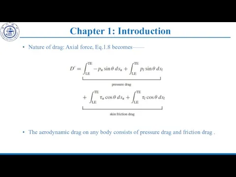
- 31. Chapter 1: Introduction Nature of drag: Axial force, Eq.1.8 becomes—— The aerodynamic drag on any body
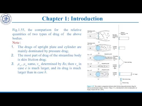
- 32. Chapter 1: Introduction Fig.1.55, the comparison for the relative quantities of two types of drag of
- 33. Chapter 1: Introduction Thus, there are two types of typical aerodynamic shapes: Blunt body: Most part
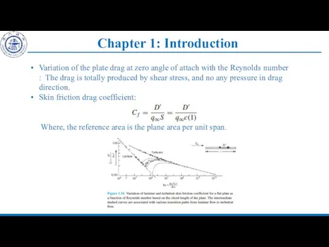
- 34. Chapter 1: Introduction Variation of the plate drag at zero angle of attach with the Reynolds
- 35. Chapter 1: Introduction The figure listed above indicates that: Cf strongly depends on Re, of which
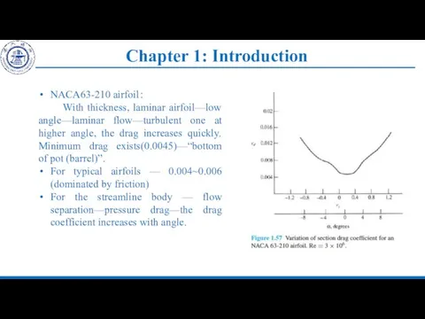
- 36. Chapter 1: Introduction NACA63-210 airfoil: With thickness, laminar airfoil—low angle—laminar flow—turbulent one at higher angle, the
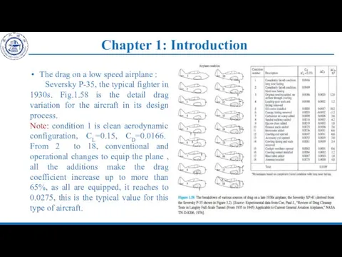
- 37. Chapter 1: Introduction The drag on a low speed airplane : Seversky P-35, the typical fighter
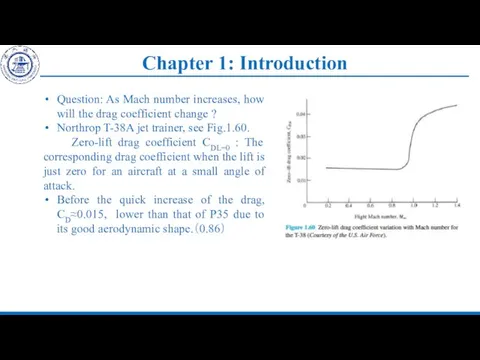
- 38. Chapter 1: Introduction Question: As Mach number increases, how will the drag coefficient change ? Northrop
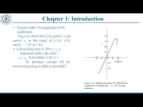
- 39. Chapter 1: Introduction Typical order of magnitude of lift coefficient: Fig.1.61-NACA63-210 airfoil ‘s lift curve—cl in
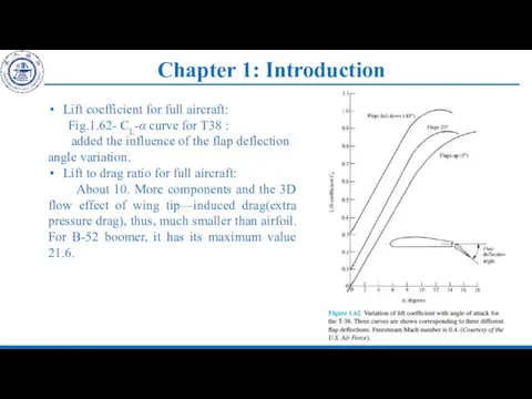
- 40. Chapter 1: Introduction Lift coefficient for full aircraft: Fig.1.62- CL-α curve for T38 : added the
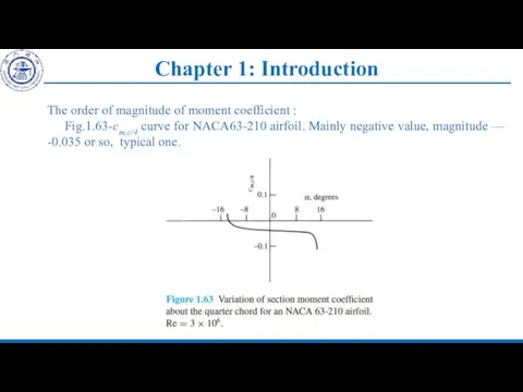
- 41. Chapter 1: Introduction The order of magnitude of moment coefficient : Fig.1.63-cm.c/4 curve for NACA63-210 airfoil.
- 42. Chapter 1: Introduction Homework: p1.16、p1.18 Thinking work: Can all the drag come down to pressure drag
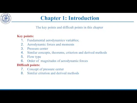
- 43. Chapter 1: Introduction The key points and difficult points in this chapter Key points: Fundamental aerodynamics
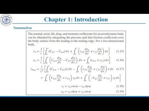
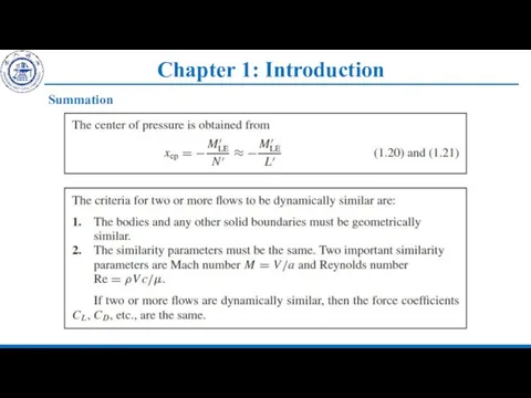
- 44. Chapter 1: Introduction Summation
- 45. Chapter 1: Introduction Summation
- 47. Скачать презентацию

Useful Info
Useful Info

Review
The Principle of Dimensional Homogeneity (PDH)——a rule which is almost a
Review
The Principle of Dimensional Homogeneity (PDH)——a rule which is almost a
Review
Basic Theorem
Review
Basic Theorem
Review
Flow similarity
By definition, different flows are dynamically similar if:
The streamline patterns
Review
Flow similarity
By definition, different flows are dynamically similar if:
The streamline patterns
Chapter 1: Introduction
Schematic of the variable density tunnel (VDT) (From Baals,
Chapter 1: Introduction
Schematic of the variable density tunnel (VDT) (From Baals,
Review
Fluid static dynamics: Buoyance
Consider the forces along y axis: Positive upward,
Review
Fluid static dynamics: Buoyance
Consider the forces along y axis: Positive upward,
Review
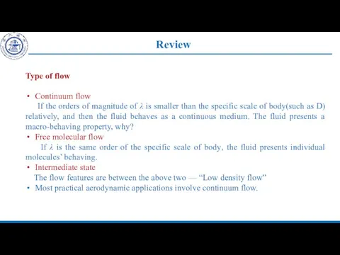
Type of flow
Continuum flow
If the orders of magnitude of λ
Review
Type of flow
Continuum flow
If the orders of magnitude of λ
Review
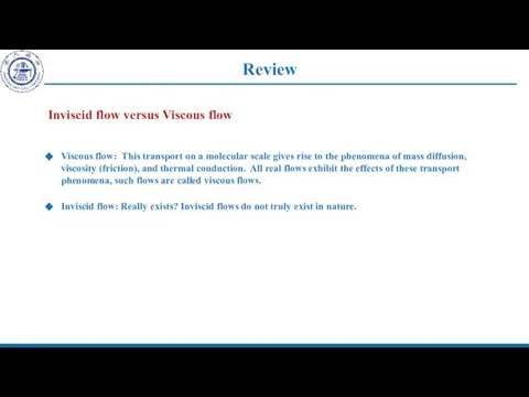
Inviscid flow versus Viscous flow
Viscous flow: This transport on a molecular
Review
Inviscid flow versus Viscous flow
Viscous flow: This transport on a molecular
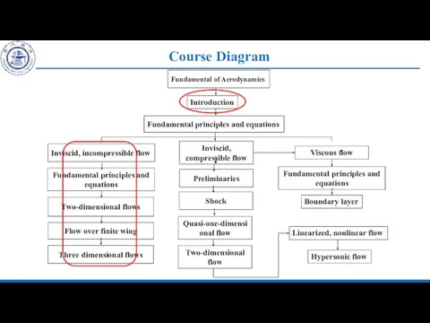
Course Diagram
Course Diagram
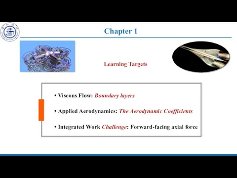
Chapter 1
Learning Targets
Chapter 1
Learning Targets
Chapter 1: Introduction
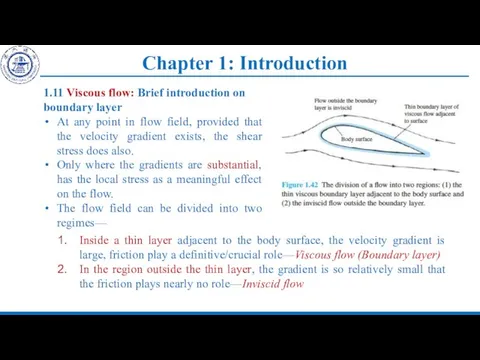
1.11 Viscous flow: Brief introduction on boundary layer
At any
Chapter 1: Introduction
1.11 Viscous flow: Brief introduction on boundary layer
At any
Chapter 1: Introduction
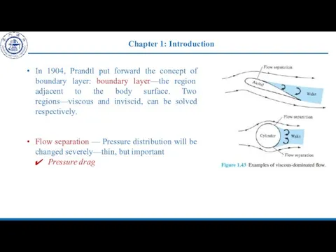
In 1904, Prandtl put forward the concept of boundary
Chapter 1: Introduction
In 1904, Prandtl put forward the concept of boundary
Chapter 1: Introduction
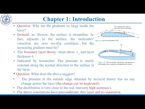
Question: Why are the gradients so large inside the
Chapter 1: Introduction
Question: Why are the gradients so large inside the
Chapter 1: Introduction
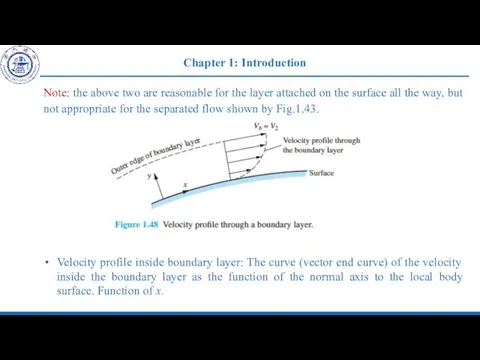
Note: the above two are reasonable for the layer
Chapter 1: Introduction
Note: the above two are reasonable for the layer
Chapter 1: Introduction
Temperature profile through the layer: The curve of the
Chapter 1: Introduction
Temperature profile through the layer: The curve of the
Chapter 1: Introduction
μ variation with temperature: liquid (olive ; soybean- edible
Chapter 1: Introduction
μ variation with temperature: liquid (olive ; soybean- edible
Chapter 1: Introduction
At standard sea level temperature:
k=2.53×10⁻²J/(m)(s)(K)
Proportional to the viscous
Chapter 1: Introduction
At standard sea level temperature:
k=2.53×10⁻²J/(m)(s)(K)
Proportional to the viscous
Chapter 1: Introduction
Re effect on boundary layer:
Figure below: Development of boundary
Chapter 1: Introduction
Re effect on boundary layer:
Figure below: Development of boundary
Chapter 1: Introduction
The Reynolds number generally governs the nature of the
Chapter 1: Introduction
The Reynolds number generally governs the nature of the
Chapter 1: Introduction
Fig.1.53: Comparison for the two velocity profiles——
Turbulent, relatively “plump”;
Laminar,
Chapter 1: Introduction
Fig.1.53: Comparison for the two velocity profiles——
Turbulent, relatively “plump”;
Laminar,
Chapter 1: Introduction
By Eq.1.59: (τw)laminer<(τw)turbulent
The important fact: The shear stress
Chapter 1: Introduction
By Eq.1.59: (τw)laminer<(τw)turbulent
The important fact: The shear stress

Chapter 1: Introduction
Homework: 1.11, 1.12
Questions for thinking:
1. After released, the
Chapter 1: Introduction
Homework: 1.11, 1.12
Questions for thinking:
1. After released, the

Chapter 1: Introduction
1.12 Applied aerodynamics: Aerodynamic coefficients——
Magnitudes and variations
Applied aerodynamics:
Chapter 1: Introduction
1.12 Applied aerodynamics: Aerodynamic coefficients——
Magnitudes and variations
Applied aerodynamics:

Chapter 1: Introduction
Lift, Drag and moment coefficient are the most frequently
Chapter 1: Introduction
Lift, Drag and moment coefficient are the most frequently
Chapter 1: Introduction
Fig.1.54, Typical drag coefficients of some bodies (fixed attitude)
Chapter 1: Introduction
Fig.1.54, Typical drag coefficients of some bodies (fixed attitude)
Chapter 1: Introduction
Comparisons between Case b and d :
One order
Chapter 1: Introduction
Comparisons between Case b and d :
One order
Chapter 1: Introduction
Comparisons between Case c and d :
Same dynamic pressures,
Chapter 1: Introduction
Comparisons between Case c and d :
Same dynamic pressures,
Chapter 1: Introduction
Comparisons between Case b and e :
Same diameter, but
Chapter 1: Introduction
Comparisons between Case b and e :
Same diameter, but
Chapter 1: Introduction
Note:Character parameter(per unit span)—the maximum windward cross-sectional area. The
Chapter 1: Introduction
Note:Character parameter(per unit span)—the maximum windward cross-sectional area. The
Chapter 1: Introduction
Nature of drag: Axial force, Eq.1.8 becomes——
The aerodynamic drag
Chapter 1: Introduction
Nature of drag: Axial force, Eq.1.8 becomes——
The aerodynamic drag
Chapter 1: Introduction
Fig.1.55, the comparison for the relative quantities of two
Chapter 1: Introduction
Fig.1.55, the comparison for the relative quantities of two

Chapter 1: Introduction
Thus, there are two types of typical aerodynamic shapes:
Blunt
Chapter 1: Introduction
Thus, there are two types of typical aerodynamic shapes:
Blunt
Chapter 1: Introduction
Variation of the plate drag at zero angle of
Chapter 1: Introduction
Variation of the plate drag at zero angle of

Chapter 1: Introduction
The figure listed above indicates that:
Cf strongly depends on
Chapter 1: Introduction
The figure listed above indicates that:
Cf strongly depends on
Chapter 1: Introduction
NACA63-210 airfoil:
With thickness, laminar airfoil—low angle—laminar flow—turbulent one
Chapter 1: Introduction
NACA63-210 airfoil:
With thickness, laminar airfoil—low angle—laminar flow—turbulent one
Chapter 1: Introduction
The drag on a low speed airplane :
Chapter 1: Introduction
The drag on a low speed airplane :
Chapter 1: Introduction
Question: As Mach number increases, how will the drag
Chapter 1: Introduction
Question: As Mach number increases, how will the drag
Chapter 1: Introduction
Typical order of magnitude of lift coefficient:
Fig.1.61-NACA63-210 airfoil
Chapter 1: Introduction
Typical order of magnitude of lift coefficient:
Fig.1.61-NACA63-210 airfoil
Chapter 1: Introduction
Lift coefficient for full aircraft:
Fig.1.62- CL-α curve for
Chapter 1: Introduction
Lift coefficient for full aircraft:
Fig.1.62- CL-α curve for
Chapter 1: Introduction
The order of magnitude of moment coefficient :
Fig.1.63-cm.c/4
Chapter 1: Introduction
The order of magnitude of moment coefficient :
Fig.1.63-cm.c/4

Chapter 1: Introduction
Homework: p1.16、p1.18
Thinking work:
Can all the drag
Chapter 1: Introduction
Homework: p1.16、p1.18
Thinking work:
Can all the drag
Chapter 1: Introduction
The key points and difficult points in this chapter
Key
Chapter 1: Introduction
The key points and difficult points in this chapter
Key
Chapter 1: Introduction
Summation
Chapter 1: Introduction
Summation
Chapter 1: Introduction
Summation
Chapter 1: Introduction
Summation
 Физика и безопасность дорожного движения
 Закон сохранения энергии
 Освещение. Свет и тень
 Великий инженер Василий Григорьевич Шухов Авторы: учащиеся 8 «Б» класса МОУ «Киришский лицей» Ленинградская область г. Кириши
  Токопроводящие пластмассы
 Тема: «Мир звука». Выполнила: ученица 11 «А» класса МОУ «СОШ № 95 им. Н. Щукина п.Архара» Сахнова Ольга Александровна.
 Влияние излучения на прорастание семян
 Презентация по физике "Строение ядра" - скачать
 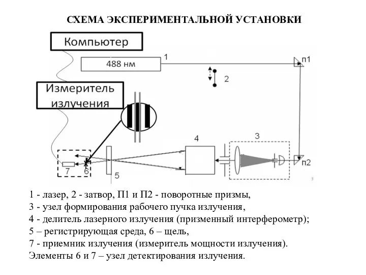 Схема экспериментальной установки
 8 класс 2009
 История и основные понятия науки о материалах
 Сорбционные процессы. (Лекция 2)
 Равновесие тел урок физики, 10 класс
  Производство передачи и использование электрической энергии
 Фізичні терміни. Атом
 Для 10 класса (базовый уровень) Учитель МБОУ СОШ № 151 Кравцова И.А.
  Теория Большого Взрыва. The Big Bang Theory
 Радиоактивность. История открытия
 Химическая эволюция и биогенез
 Ядерний реактор Будова та принцип дії
  Кипение. Испарение
 Лекция 12
  Фундаментальные опыты в оптике
 Виды излучений
 Деформация и механические свойства материалов
 Постоянный электрический ток. Причины электрического тока
 Строение атома
 Презентация по физике Законы Ньютона