- Back propagation example

Содержание
- 2. 20 Error .90 .17 1 .76 1.0 0.0 1 4.5 -5.2 -2.0 -4.6 -1.5 3.7 2.9
- 3. 21 Key Concepts Gradient descent error is a function of the weights we want to reduce
- 4. 22 Gradient Descent λ error(λ) gradient = 1 current λ optimal λ
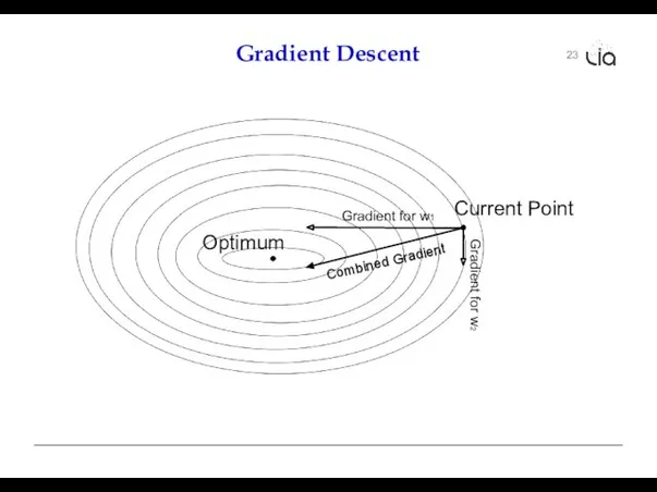
- 5. 23 Gradient Descent Gradient for w1 Gradient for w2 Optimum Current Point Combined Gradient
- 6. Coborârea gradientului (gradient descent) în spațiul ponderilor Din cartea Machine Learning, de Tom Mitchel. http://profsite.um.ac.ir/~monsefi/machine-learning/pdf/Machine-Learning-Tom-Mitchell.pdf
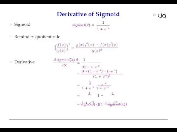
- 7. 24 Derivative of Sigmoid Sigmoid 1 sigmoid(x) = 1 + e−x Reminder: quotient rule Derivative dx
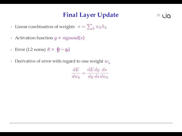
- 8. 25 Final Layer Update Linear combination of weights Activation function y = sigmoid(s) 2 Error (L2
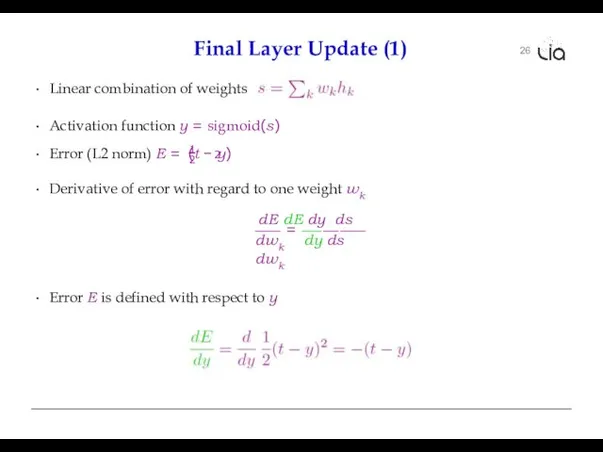
- 9. 26 Final Layer Update (1) 2 Error (L2 norm) E = (t − y) 1 2
- 10. 27 Final Layer Update (2) Linear combination of weights Activation function y = sigmoid(s) 2 Error
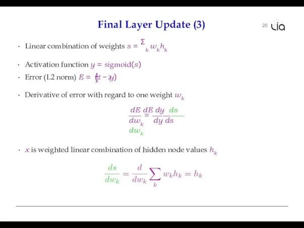
- 11. 28 Final Layer Update (3) Linear combination of weights s = Σk wkhk Activation function y
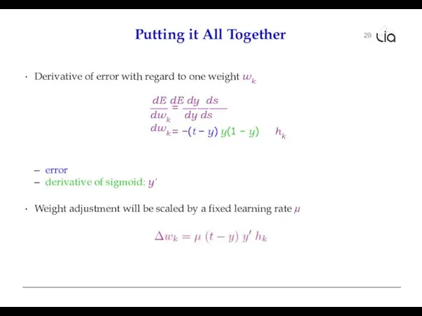
- 12. 29 Putting it All Together Derivative of error with regard to one weight wk = dE
- 13. 30 Multiple Output Nodes Our example only had one output node Typically neural networks have multiple
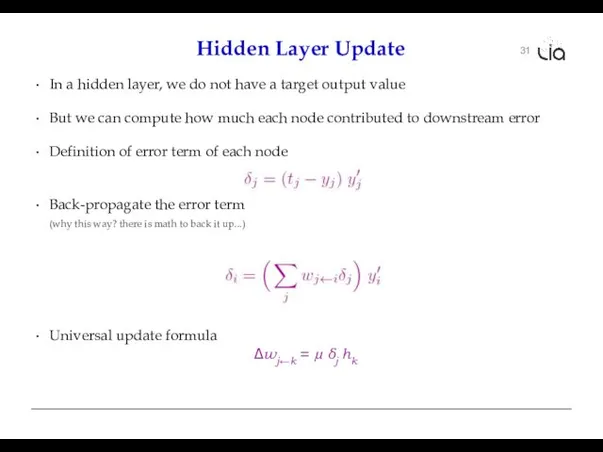
- 14. 31 Hidden Layer Update In a hidden layer, we do not have a target output value
- 15. 32 Our Example .17 4.5 -5.2 -2.0 -4.6 -1.5 2.9 3.7 2.9 A 1.0 B 0.0
- 16. 33 Our Example .17 -4.6 -1.5 2.9 3.7 2.9 A 1.0 B 0.0 C 1 3.7
- 17. 34 Hidden Layer Updates .17 -4.6 -1.5 2.9 3.7 2.9 A 1.0 B 0.0 C 1
- 18. 35 some additional aspects
- 19. 36 Initialization of Weights Weights are initialized randomly e.g., uniformly from interval [−0.01, 0.01] Glorot and
- 20. 37 Neural Networks for Classification Predict class: one output node per class Training data output: ”One-hot
- 21. 38 Problems with Gradient Descent Training error(λ) λ Too high learning rate
- 22. 39 Problems with Gradient Descent Training error(λ) λ Bad initialization Philipp Koehn Machine Translation: Introduction to
- 23. 40 Problems with Gradient Descent Training λ error(λ) local optimum global optimum Local optimum
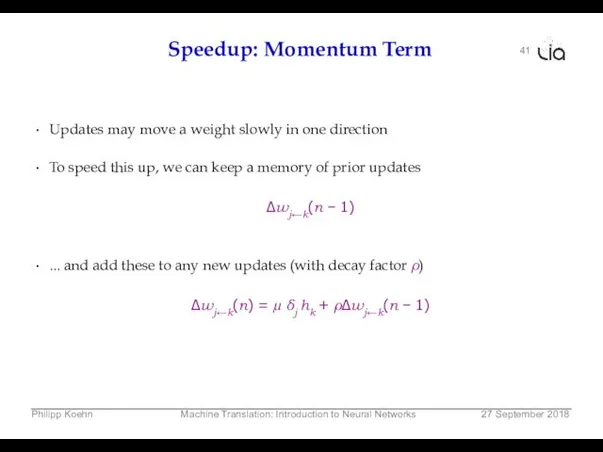
- 24. 41 Speedup: Momentum Term Updates may move a weight slowly in one direction To speed this
- 25. 42 Adagrad Typically reduce the learning rate µ over time at the beginning, things have to
- 26. 43 Dropout A general problem of machine learning: overfitting to training data (very good on train,
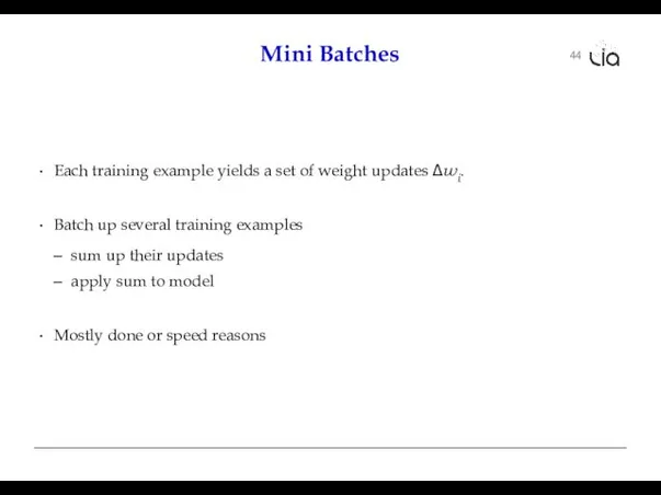
- 27. 44 Mini Batches Each training example yields a set of weight updates ∆wi. Batch up several
- 28. 45 computational aspects
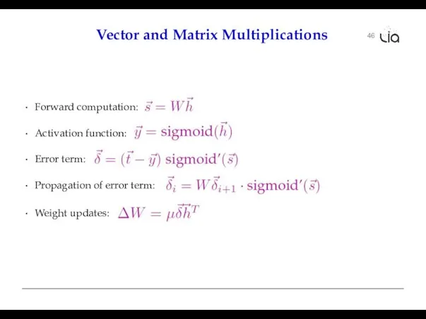
- 29. 46 Vector and Matrix Multiplications Forward computation: Activation function: Error term: Propagation of error term: Weight
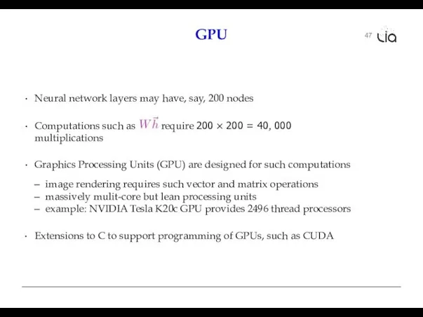
- 30. 47 GPU Neural network layers may have, say, 200 nodes Computations such as require 200 ×
- 31. 48 Toolkits Theano Tensorflow (Google) PyTorch (Facebook) MXNet (Amazon) DyNet С (easy api)
- 32. lia@math.md
- 34. Скачать презентацию

20
Error
.90
.17
1
.76
1.0
0.0
1
4.5
-5.2
-2.0
-4.6
-1.5
3.7
2.9
3.7
2.9
Computed output: y = .76
Correct output: t = 1.0
⇒
20
Error
.90
.17
1
.76
1.0
0.0
1
4.5
-5.2
-2.0
-4.6
-1.5
3.7
2.9
3.7
2.9
Computed output: y = .76
Correct output: t = 1.0
⇒

21
Key Concepts
Gradient descent
error is a function of the weights
we want to
21
Key Concepts
Gradient descent
error is a function of the weights
we want to

22
Gradient Descent
λ
error(λ)
gradient = 1
current λ
optimal λ
22
Gradient Descent
λ
error(λ)
gradient = 1
current λ
optimal λ
23
Gradient Descent
Gradient for w1
Gradient for w2
Optimum
Current Point
Combined Gradient
23
Gradient Descent
Gradient for w1
Gradient for w2
Optimum
Current Point
Combined Gradient
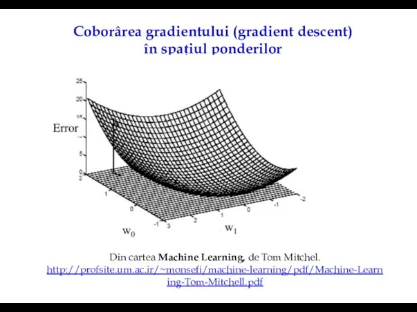
Coborârea gradientului (gradient descent) în spațiul ponderilor
Din cartea Machine Learning, de
Coborârea gradientului (gradient descent) în spațiul ponderilor
Din cartea Machine Learning, de
24
Derivative of Sigmoid
Sigmoid
1
sigmoid(x) =
1 + e−x
Reminder: quotient rule
Derivative
dx
d sigmoid(x) d 1
=
dx 1 +
24
Derivative of Sigmoid
Sigmoid
1
sigmoid(x) =
1 + e−x
Reminder: quotient rule
Derivative
dx
d sigmoid(x) d 1
=
dx 1 +
25
Final Layer Update
Linear combination of weights
Activation function y = sigmoid(s)
2
Error
25
Final Layer Update
Linear combination of weights
Activation function y = sigmoid(s)
2
Error
26
Final Layer Update (1)
2
Error (L2 norm) E = (t − y)
1 2
Derivative of
26
Final Layer Update (1)
2
Error (L2 norm) E = (t − y)
1 2
Derivative of

27
Final Layer Update (2)
Linear combination of weights
Activation function y =
27
Final Layer Update (2)
Linear combination of weights
Activation function y =
28
Final Layer Update (3)
Linear combination of weights s = Σk wkhk
Activation
28
Final Layer Update (3)
Linear combination of weights s = Σk wkhk
Activation
29
Putting it All Together
Derivative of error with regard to one weight
29
Putting it All Together
Derivative of error with regard to one weight

30
Multiple Output Nodes
Our example only had one output node
Typically neural networks
30
Multiple Output Nodes
Our example only had one output node
Typically neural networks
31
Hidden Layer Update
In a hidden layer, we do not have a
31
Hidden Layer Update
In a hidden layer, we do not have a
32
Our Example
.17
4.5
-5.2
-2.0
-4.6
-1.5
2.9
3.7
2.9
A
1.0
B
0.0
C
1
3.7 D
.90
E
F
1
G
.76
Computed output: y = .76
Correct output: t =
32
Our Example
.17
4.5
-5.2
-2.0
-4.6
-1.5
2.9
3.7
2.9
A
1.0
B
0.0
C
1
3.7 D
.90
E
F
1
G
.76
Computed output: y = .76
Correct output: t =

33
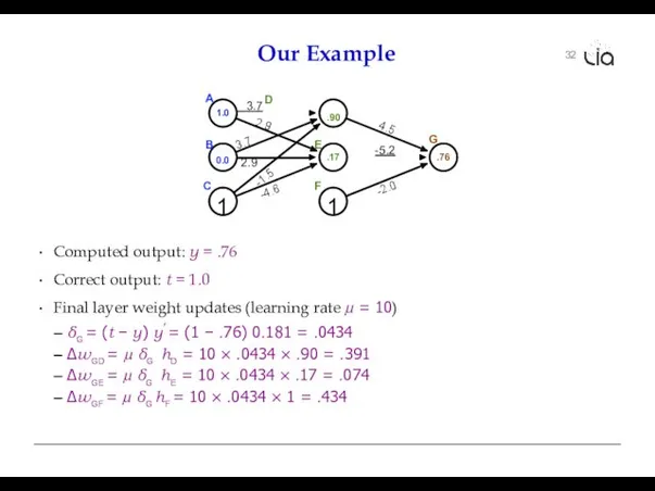
Our Example
.17
-4.6
-1.5
2.9
3.7
2.9
A
1.0
B
0.0
C
1
3.7 D
.90
E
F
1
G
.76
4.8914—.5
-5.126 -—5.—2
-1.566 —-2.—0
Computed output: y = .76
Correct output: t
33
Our Example
.17
-4.6
-1.5
2.9
3.7
2.9
A
1.0
B
0.0
C
1
3.7 D
.90
E
F
1
G
.76
4.8914—.5
-5.126 -—5.—2
-1.566 —-2.—0
Computed output: y = .76
Correct output: t

34
Hidden Layer Updates
.17
-4.6
-1.5
2.9
3.7
2.9
A
1.0
B
0.0
C
1
3.7 D
.90
E
F
1
G
.76
4.8914—.5
-5.126 -—5.—2
-1.566 —-2.—0
Hidden node D
Hidden node E
34
Hidden Layer Updates
.17
-4.6
-1.5
2.9
3.7
2.9
A
1.0
B
0.0
C
1
3.7 D
.90
E
F
1
G
.76
4.8914—.5
-5.126 -—5.—2
-1.566 —-2.—0
Hidden node D
Hidden node E

35
some additional aspects
35
some additional aspects

36
Initialization of Weights
Weights are initialized randomly
e.g., uniformly from interval [−0.01, 0.01]
Glorot
36
Initialization of Weights
Weights are initialized randomly
e.g., uniformly from interval [−0.01, 0.01]
Glorot
37
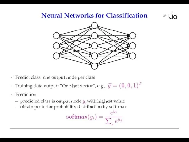
Neural Networks for Classification
Predict class: one output node per class
Training data
37
Neural Networks for Classification
Predict class: one output node per class
Training data
38
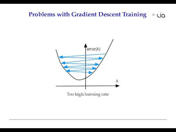
Problems with Gradient Descent Training
error(λ)
λ
Too high learning rate
38
Problems with Gradient Descent Training
error(λ)
λ
Too high learning rate
39
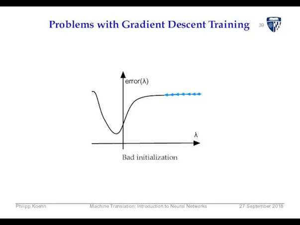
Problems with Gradient Descent Training
error(λ)
λ
Bad initialization
Philipp Koehn
Machine Translation: Introduction to Neural
39
Problems with Gradient Descent Training
error(λ)
λ
Bad initialization
Philipp Koehn
Machine Translation: Introduction to Neural

40
Problems with Gradient Descent Training
λ
error(λ)
local optimum
global optimum
Local optimum
40
Problems with Gradient Descent Training
λ
error(λ)
local optimum
global optimum
Local optimum
41
Speedup: Momentum Term
Updates may move a weight slowly in one direction
To
41
Speedup: Momentum Term
Updates may move a weight slowly in one direction
To

42
Adagrad
Typically reduce the learning rate µ over time
at the beginning, things
42
Adagrad
Typically reduce the learning rate µ over time
at the beginning, things

43
Dropout
A general problem of machine learning: overfitting to training data (very
43
Dropout
A general problem of machine learning: overfitting to training data (very
44
Mini Batches
Each training example yields a set of weight updates ∆wi.
Batch
44
Mini Batches
Each training example yields a set of weight updates ∆wi.
Batch

45
computational aspects
45
computational aspects
46
Vector and Matrix Multiplications
Forward computation:
Activation function:
Error term:
Propagation of error
46
Vector and Matrix Multiplications
Forward computation:
Activation function:
Error term:
Propagation of error
47
GPU
Neural network layers may have, say, 200 nodes
Computations such as require
47
GPU
Neural network layers may have, say, 200 nodes
Computations such as require

48
Toolkits
Theano
Tensorflow (Google)
PyTorch (Facebook)
MXNet (Amazon)
DyNet
С (easy api)
48
Toolkits
Theano
Tensorflow (Google)
PyTorch (Facebook)
MXNet (Amazon)
DyNet
С (easy api)

lia@math.md
lia@math.md
 Создание слайд-шоу. Фотоальбом. Урок 29
 SQL запросы
 Лекция 12. Двусторонняя очередь: deque. Адаптеры контейнеров: stack, queue, priority_queue. Создание DLL
 Действия с информацией
 Проектирование Баз Данных. Основные понятия Теории Нормализации
 Презентация к уроку информатики по теме «Растровое кодирование графической информации» Автор: Смелова Наталья Александровна, уч
 Что умеет компьютер
 Использование систем проверки орфографии и грамматики
 Нормальные формы баз данных
 Графический дизайн. Компьютерная графика
 Метод координат
 Общая концепция. Поиск по всей базе данных
 Требования к специалистам строительных организаций. Национальный реестр специалистов строительной отрасли
 Алгоритм с ветвлением
 Инфологическая модель БД
 Лекция № 15. Поиск и индексация
 Использование график, таблиц, диаграмм в презентации. Лабораторная работа № 3
 Архитектура компьютера Презентацию выполнила студентка 1 курса Ермакова Ольга
 Экспертные системы
 Создание документов на базе комплекса программных средств электронного офиса Microsoft Office
 Язык С# как современная альтернатива Паскалю и С++ для обучения основам алгоритмизации и программирования Павловская Татьяна А
 Тезисы. Доклад. Презентация. Всё о конференциях
 Строки в языке программирования C++
 Мобильная медиашкола
 Как устроен компьютер
 Лексические основы, арифметические типы данных, переменные и константы, операторы, линейный алгоритм. (Семинар 1)
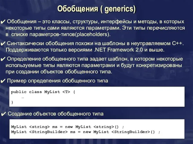 Обобщения
 Аттестационная работа. Творческие проекты в среде программирования скретч, для 5-6 класса