Discrete random variables – expected variance and standard deviation. Discrete Probability Distributions. Week 7 (1)
- Discrete random variables – expected variance and standard deviation. Discrete Probability Distributions. Week 7 (1)

Содержание
- 2. DR SUSANNE HANSEN SARAL
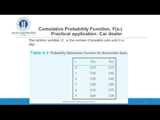
- 3. Cumulative Probability Function, F(x0) Practical application: Car dealer DR SUSANNE HANSEN SARAL The random variable, X,
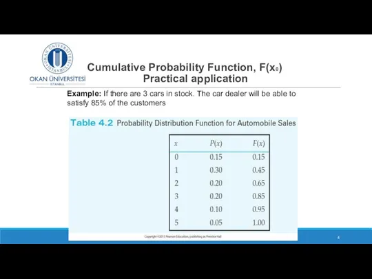
- 4. Cumulative Probability Function, F(x0) Practical application DR SUSANNE HANSEN SARAL Example: If there are 3 cars
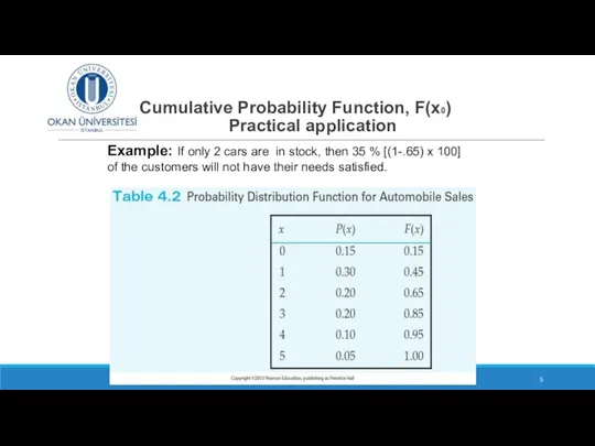
- 5. Cumulative Probability Function, F(x0) Practical application DR SUSANNE HANSEN SARAL Example: If only 2 cars are
- 6. Properties of discrete random variables: Expected value E[x] = (0 x .25) + (1 x .50)
- 7. Expected value for a discrete random variable Exercise X is a discrete random variable. The graph
- 8. Expected value for a discrete random variable X is a discrete random variable. The graph below
- 9. Expected variance of a Discrete Random Variables DR SUSANNE HANSEN SARAL
- 10. Variance of a discrete random variable DR SUSANNE HANSEN SARAL
- 11. Variance and Standard Deviation Ch. 4- DR SUSANNE HANSEN SARAL
- 12. At a car dealer the number of cars sold daily could vary between 0 and 5
- 13. Calculation of variance of discrete random variable. Car sales – example DR SUSANNE HANSEN SARAL
- 14. Class exercise A car dealer calculates the proportion of new cars sold that have been returned
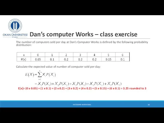
- 15. Dan’s computer Works – class exercise The number of computers sold per day at Dan’s Computer
- 16. Dan’s computer Works – class exercise The number of computers sold per day at Dan’s Computer
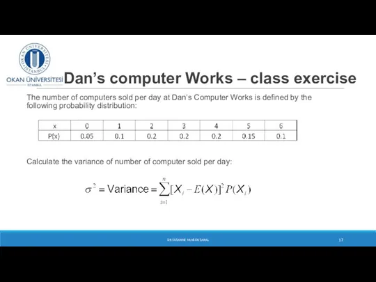
- 17. Dan’s computer Works – class exercise The number of computers sold per day at Dan’s Computer
- 18. Dan’s computer Works – class exercise DR SUSANNE HANSEN SARAL
- 19. Quizz A small school employs 5 teachers who make between $40,000 and $70,000 per year. One
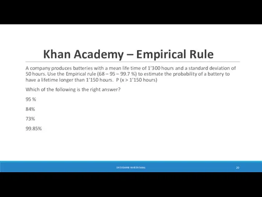
- 20. Khan Academy – Empirical Rule A company produces batteries with a mean life time of 1’300
- 21. Stating that two events are statistically independent means that the probability of one event occurring is
- 22. The time it takes a car to drive from Istanbul to Sinop is an example of
- 23. Probability is a numerical measure about the likelihood that an event will occur. TRUE FALSE
- 24. Suppose that you enter a lottery by obtaining one of 20 tickets that have been distributed.
- 25. If we flip a coin three times, the probability of getting three heads is 0.125. TRUE
- 26. The number of products bought at a local store is an example of a discrete random
- 27. Empirical rule – Khan Academy a) Which shape does a distribution need to have to apply
- 28. Probability Distributions Continuous Probability Distributions Binomial Probability Distributions Discrete Probability Distributions Uniform Normal Exponential DR SUSANNE
- 29. Binomial Probability Distribution Bi-nominal (from Latin) means: Two-names A fixed number of observations, n e.g., 15
- 30. Possible Binomial Distribution examples A manufacturing plant labels products as either defective or acceptable A firm
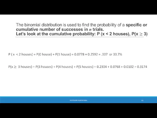
- 31. The Binomial Distribution The binomial distribution is used to find the probability of a specific or
- 32. The Binomial Distribution The binomial formula is: 2 – The symbol ! means factorial, and n!
- 33. Example: Calculating a Binomial Probability What is the probability of one success in five observations if
- 34. Binomial probability - Calculating binomial probabilities Suppose that Ali, a real estate agent, has 5 people
- 35. Solving Problems with the Binomial Formula Find the probability of 4 people buying a house out
- 36. Class exerise Find the probability of 3 people buying a house out of 5 people, when
- 37. P( X = 3) ? Find the probability of 3 people buying a house out of
- 38. Creating a probability distribution with the Binomial Formula – house sale example 2 – TABLE 2.8
- 39. Binomial Probability Distribution house sale example n = 5, P= .4 DR SUSANNE HANSEN SARAL
- 40. DR SUSANNE HANSEN SARAL
- 41. DR SUSANNE HANSEN SARAL
- 42. Shape of Binomial Distribution The shape of the binomial distribution depends on the values of P
- 43. Binomial Distribution shapes When P = .5 the shape of the distribution is perfectly symmetrical and
- 44. Using Binomial Tables instead of to calculating Binomial probabilites DR SUSANNE HANSEN SARAL Ch. 4- Examples:
- 45. Solving Problems with Binomial Tables MSA Electronics is experimenting with the manufacture of a new USB-stick
- 47. Скачать презентацию
DR SUSANNE HANSEN SARAL
DR SUSANNE HANSEN SARAL
Cumulative Probability Function, F(x0)
Practical application: Car dealer
DR SUSANNE HANSEN
Cumulative Probability Function, F(x0)
Practical application: Car dealer
DR SUSANNE HANSEN
Cumulative Probability Function, F(x0)
Practical application
DR SUSANNE HANSEN SARAL
Example: If
Cumulative Probability Function, F(x0)
Practical application
DR SUSANNE HANSEN SARAL
Example: If
Cumulative Probability Function, F(x0)
Practical application
DR SUSANNE HANSEN SARAL
Example: If
Cumulative Probability Function, F(x0)
Practical application
DR SUSANNE HANSEN SARAL
Example: If
![Properties of discrete random variables: Expected value E[x] = (0 x](/_ipx/f_webp&q_80&fit_contain&s_1440x1080/imagesDir/jpg/1465184/slide-5.jpg)
Properties of discrete random variables: Expected value
E[x] = (0
Properties of discrete random variables: Expected value
E[x] = (0
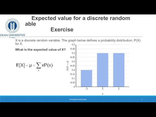
Expected value for a discrete random variable
Exercise
X is a discrete
Expected value for a discrete random variable
Exercise
X is a discrete
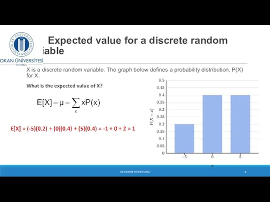
Expected value for a discrete random variable
X is a discrete random
Expected value for a discrete random variable
X is a discrete random
Expected variance
of a Discrete Random Variables
DR SUSANNE HANSEN SARAL
Expected variance
of a Discrete Random Variables
DR SUSANNE HANSEN SARAL
Variance of a discrete random variable
DR SUSANNE HANSEN SARAL
Variance of a discrete random variable
DR SUSANNE HANSEN SARAL
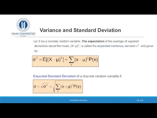
Variance and Standard Deviation
Ch. 4-
DR SUSANNE HANSEN SARAL
Variance and Standard Deviation
Ch. 4-
DR SUSANNE HANSEN SARAL
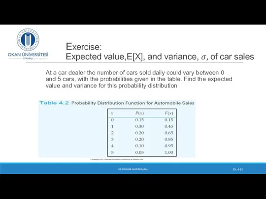
At a car dealer the number of cars sold daily could
At a car dealer the number of cars sold daily could
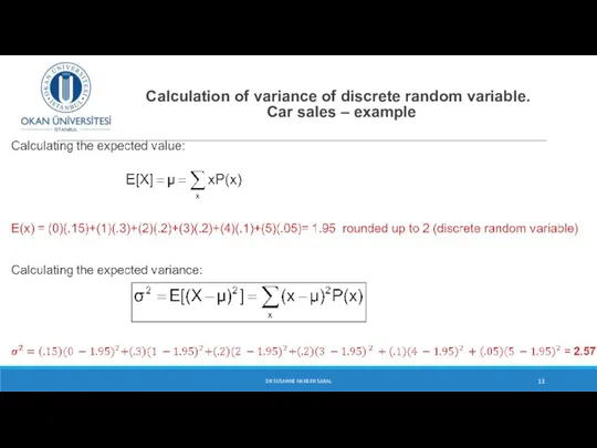
Calculation of variance of discrete random variable. Car sales –
Calculation of variance of discrete random variable. Car sales –

Class exercise
A car dealer calculates the proportion of new cars
Class exercise
A car dealer calculates the proportion of new cars
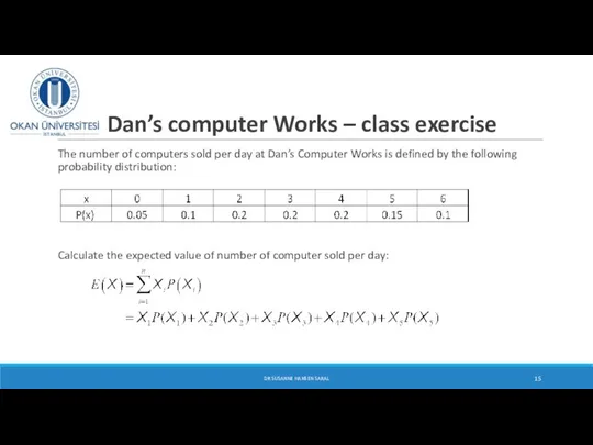
Dan’s computer Works – class exercise
The number of computers sold
Dan’s computer Works – class exercise
The number of computers sold
Dan’s computer Works – class exercise
The number of computers sold
Dan’s computer Works – class exercise
The number of computers sold
Dan’s computer Works – class exercise
The number of computers sold
Dan’s computer Works – class exercise
The number of computers sold
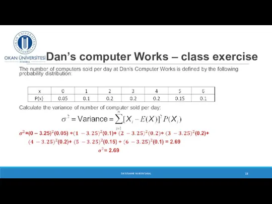
Dan’s computer Works – class exercise
DR SUSANNE HANSEN SARAL
Dan’s computer Works – class exercise
DR SUSANNE HANSEN SARAL
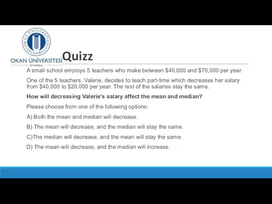
Quizz
A small school employs 5 teachers who make between $40,000 and $70,000
Quizz
A small school employs 5 teachers who make between $40,000 and $70,000
Khan Academy – Empirical Rule
A company produces batteries with a
Khan Academy – Empirical Rule
A company produces batteries with a
Stating that two events are statistically independent means that the probability
Stating that two events are statistically independent means that the probability
The time it takes a car to drive from Istanbul to
The time it takes a car to drive from Istanbul to
Probability is a numerical measure about the likelihood that an event
Probability is a numerical measure about the likelihood that an event
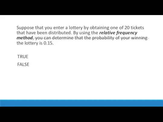
Suppose that you enter a lottery by obtaining one of 20
Suppose that you enter a lottery by obtaining one of 20
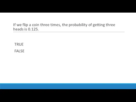
If we flip a coin three times, the probability of getting
If we flip a coin three times, the probability of getting
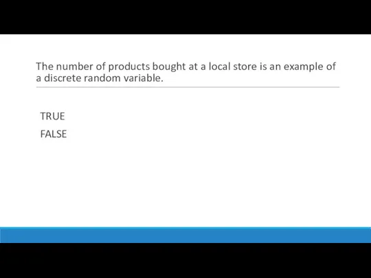
The number of products bought at a local store is an
The number of products bought at a local store is an

Empirical rule – Khan Academy
a) Which shape does a
Empirical rule – Khan Academy
a) Which shape does a
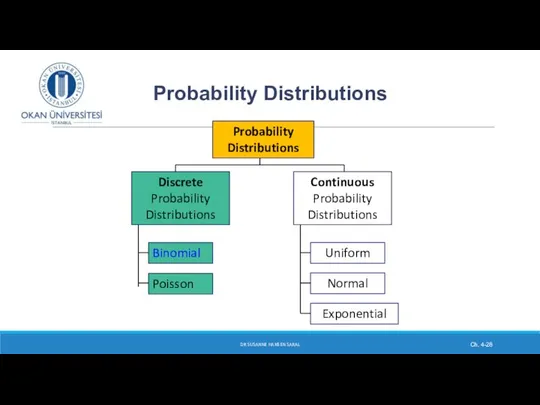
Probability Distributions
Continuous
Probability Distributions
Binomial
Probability Distributions
Discrete
Probability Distributions
Uniform
Normal
Exponential
DR SUSANNE HANSEN SARAL
Ch.
Probability Distributions
Continuous
Probability Distributions
Binomial
Probability Distributions
Discrete
Probability Distributions
Uniform
Normal
Exponential
DR SUSANNE HANSEN SARAL
Ch.

Binomial Probability Distribution
Bi-nominal (from Latin) means: Two-names
A fixed number of observations,
Binomial Probability Distribution
Bi-nominal (from Latin) means: Two-names
A fixed number of observations,
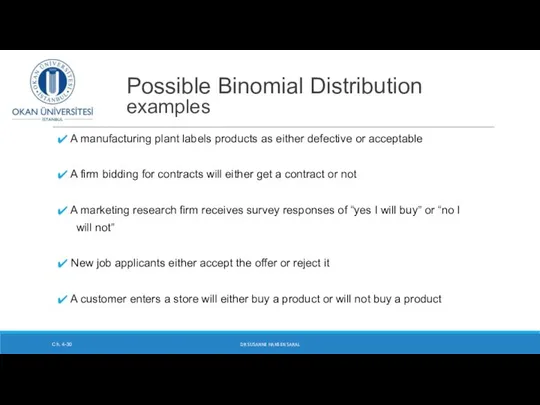
Possible Binomial Distribution
examples
A manufacturing plant labels products as either
Possible Binomial Distribution
examples
A manufacturing plant labels products as either
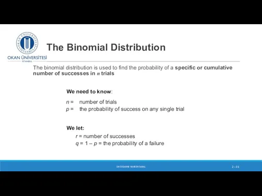
The Binomial Distribution
The binomial distribution is used to find the probability
The Binomial Distribution
The binomial distribution is used to find the probability
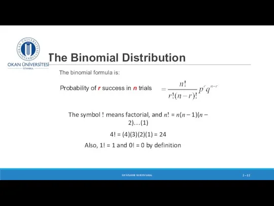
The Binomial Distribution
The binomial formula is:
2 –
The symbol ! means
The Binomial Distribution
The binomial formula is:
2 –
The symbol ! means

Example:
Calculating a Binomial Probability
What is the probability of one success
Example:
Calculating a Binomial Probability
What is the probability of one success
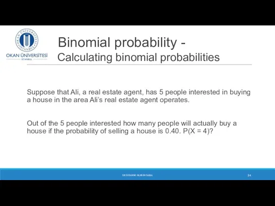
Binomial probability -
Calculating binomial probabilities
Suppose that Ali, a real
Binomial probability -
Calculating binomial probabilities
Suppose that Ali, a real
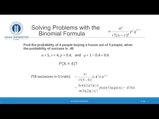
Solving Problems with the Binomial Formula
Find the probability of 4
Solving Problems with the Binomial Formula
Find the probability of 4

Class exerise
Find the probability of 3 people buying a house
Class exerise
Find the probability of 3 people buying a house

P( X = 3) ?
Find the probability of 3
P( X = 3) ?
Find the probability of 3

Creating a probability distribution with the Binomial Formula – house
Creating a probability distribution with the Binomial Formula – house

Binomial Probability Distribution
house sale example
n = 5, P=
Binomial Probability Distribution house sale example n = 5, P=

DR SUSANNE HANSEN SARAL
DR SUSANNE HANSEN SARAL
DR SUSANNE HANSEN SARAL
DR SUSANNE HANSEN SARAL
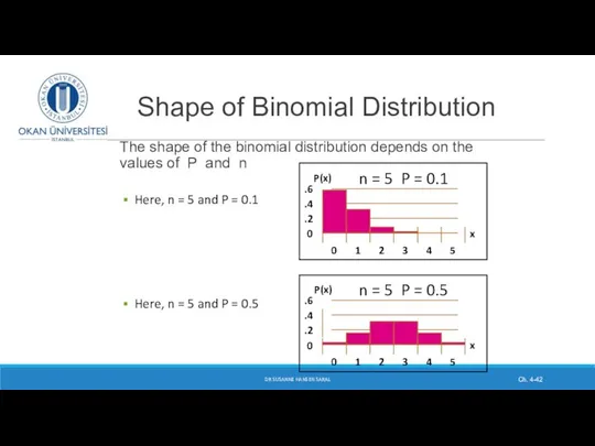
Shape of Binomial Distribution
The shape of the binomial distribution depends on
Shape of Binomial Distribution
The shape of the binomial distribution depends on

Binomial Distribution shapes
When P = .5 the shape of the
Binomial Distribution shapes
When P = .5 the shape of the

Using Binomial Tables instead of to calculating Binomial probabilites
DR SUSANNE
Using Binomial Tables instead of to calculating Binomial probabilites
DR SUSANNE
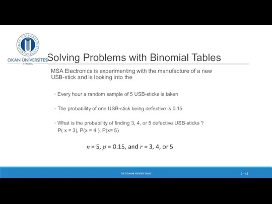
Solving Problems with Binomial Tables
MSA Electronics is experimenting with the manufacture
Solving Problems with Binomial Tables
MSA Electronics is experimenting with the manufacture
 Математика. Решение задач
 Действия с натуральными числами. Урок-сказка
 Производная сложной функции
 Начертательная геометрия. Метод проекций
 Математические ребусы. 6 класс
 Игра для 5 класса
 Действия с геометрическими фигурами, координатами и векторами
 Аксонометрическая проекция окружности
 Структурные схемы и их преобразование. Типовые динамические звенья САУ и их классификация
 Теория множеств. Понятие множества
 Заинька. Математическая раскраска. Реши примеры и покажи ответы
 Презентация по математике "Способы записи чисел" - скачать
  Екі айнымалысы бар сызықтық теңдеудің графигі
 Векторы на плоскости
 Презентация по математике "Проценты. Начальные понятия" - скачать
  Золотое сечение
 Свойства функций у = tgx и y = ctgx и их графики
 20160720_simmetriya
 Математика в поэзии
 Деление с остатком
 Вписанная и описанная окружности
 Обернена тригонометрична функція y=arcsinx
 Решение задач по теме «Площадь круга»
 Графики квадратичных функций
 Успешные люди – люди, которые в полной мере используют свой интеллект
 Применение первого признака равенства треугольников к решению задач
 «Своя игра». Внеклассное мероприятие по математике
 Автор: Галдин В. А. Учитель математики и физики МБОУ ЛСОШ №3 п. Локоть Брасовского р-на Электронная поста: galdin.vas@yandex.ru