- Model Parameterization in tomography problems. Lecture 4

Содержание
- 2. Course structure (major elements): Linearization, reducing to a system of linear equations Inversion BASIC_TOMO code: linear
- 3. Lecture 4 Model Parameterization in tomography problems Ivan Koulakov IPGG
- 4. Discretization (parameterization) Presenting the slowness distribution with a finite number of parameters (e.g., cells) System of
- 5. System of linear equations in tomography General representation: or A is the sensitivity matrix Properties of
- 6. Common myth: Number of parameters should be less than the number of data Dias N.A., et
- 7. Synthetic model Effect of grid spacing 2646 rays, all directions Smoothing: 10 Noise: 0 Grid: 1x1
- 8. Parameterization is a method for definition of a model with a finite number of parameters The
- 9. Parameterization of the 1D model Layers with constant velocities:
- 10. velocity in nodes; lineal interpolation in between Parameterization of the 1D model
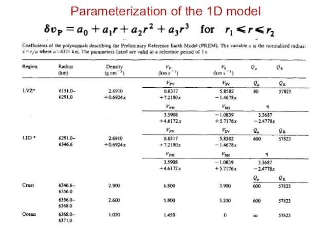
- 11. Coefficients of the Taylor series (polynomes) Parameterization of the 1D model
- 12. Parameterization of the 1D model
- 13. Parameterization of the 1D model
- 14. Parameterization of the 1D model
- 15. 3D model parameterization Three-linear interpolation x1
- 16. Parameterization Nodes of the parameterization grid are defined according to the ray distribution Between the nodes,
- 17. Model of Paleozoic complex created by the PetroTrace Company (example of a flexible manipulation with parameterization)
- 18. Travel times: observed (black) and calculated in the final velocity model (red). Rays in the starting
- 19. The target object: velocity distribution in the Paleozoic basement It is presumed that the interface geometry
- 20. Parameterization in zones: Removal links between zones makes it possible to reveal sharp contrasts in velocity
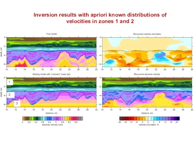
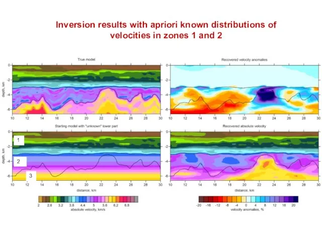
- 21. Inversion results with apriori known distributions of velocities in zones 1 and 2 1 2 3
- 22. Inversion results with apriori known distributions of velocities in zones 1 and 2 1 2 3
- 23. Results of inversions based on different starting models taking into account various apriori information no apriori
- 24. Regional model parameterization Cells in the Cartesian coordinates Performing inversions in several grids with different basic
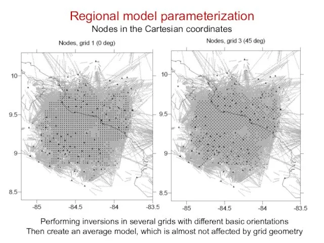
- 25. Regional model parameterization Nodes in the Cartesian coordinates Performing inversions in several grids with different basic
- 26. Adapting parameterization to the existing model information: Double-sided nodes on interfaces.
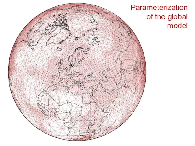
- 27. Parameterization of the global model
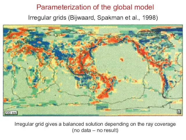
- 28. Irregular grids (Bijwaard, Spakman et al., 1998)
- 29. Irregular grid gives a balanced solution depending on the ray coverage (no data – no result)
- 30. Parameterization of the global model
- 31. Parameterization of the global model
- 32. Parameterization of the global model
- 33. Fourier series decomposition: Problem: extrapolation to areas where there are no data!
- 34. Parameterization with spherical functions Сферические функции: Расчет матрицы первых производных:
- 35. Parameterization with spherical functions
- 36. Dziewonski, 1984 Parameterization with spherical functions
- 38. Скачать презентацию
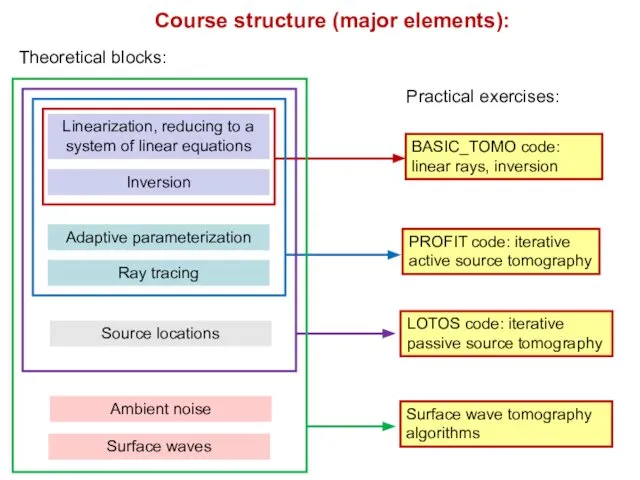
Course structure (major elements):
Linearization, reducing to a system of linear equations
Inversion
BASIC_TOMO
Course structure (major elements):
Linearization, reducing to a system of linear equations
Inversion
BASIC_TOMO
Lecture 4
Model Parameterization in tomography problems
Ivan Koulakov
IPGG
Lecture 4
Model Parameterization in tomography problems
Ivan Koulakov
IPGG
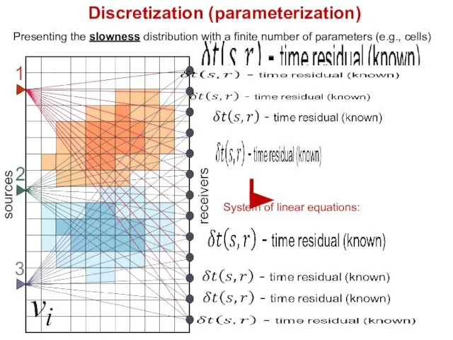
Discretization (parameterization)
Presenting the slowness distribution with a finite number of parameters
Discretization (parameterization)
Presenting the slowness distribution with a finite number of parameters
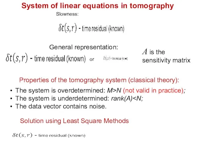
System of linear equations in tomography
General representation:
or
A is the sensitivity matrix
Properties
System of linear equations in tomography
General representation:
or
A is the sensitivity matrix
Properties
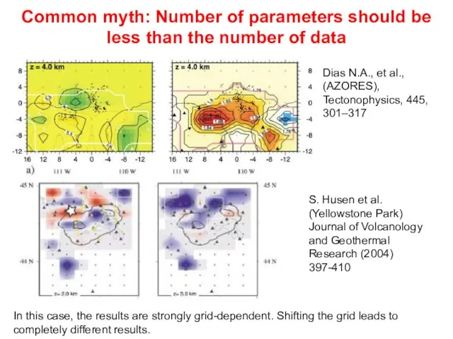
Common myth: Number of parameters should be less than the number
Common myth: Number of parameters should be less than the number
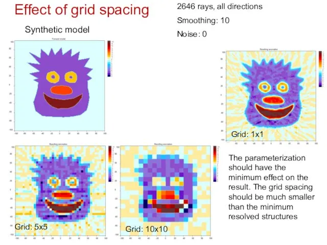
Synthetic model
Effect of grid spacing
2646 rays, all directions
Smoothing: 10
Noise: 0
Grid: 1x1
Grid:
Synthetic model
Effect of grid spacing
2646 rays, all directions
Smoothing: 10
Noise: 0
Grid: 1x1
Grid:
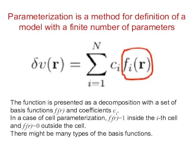
Parameterization is a method for definition of a model with a
Parameterization is a method for definition of a model with a
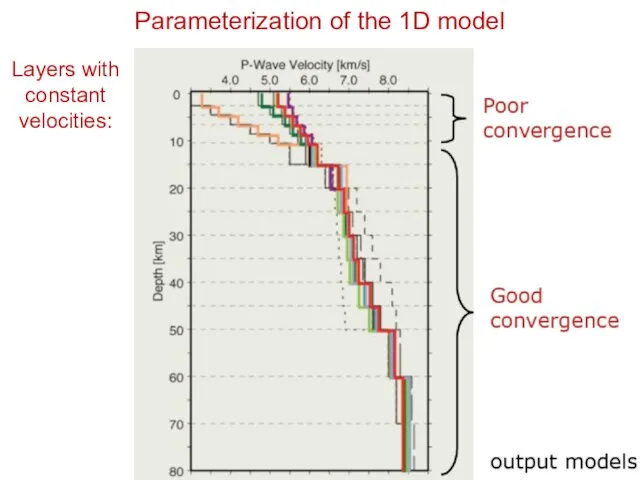
Parameterization of the 1D model
Layers with constant velocities:
Parameterization of the 1D model
Layers with constant velocities:
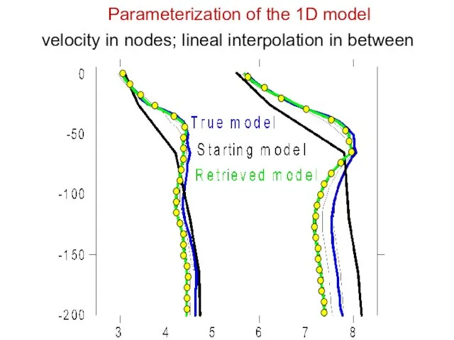
velocity in nodes; lineal interpolation in between
Parameterization of the 1D model
velocity in nodes; lineal interpolation in between
Parameterization of the 1D model
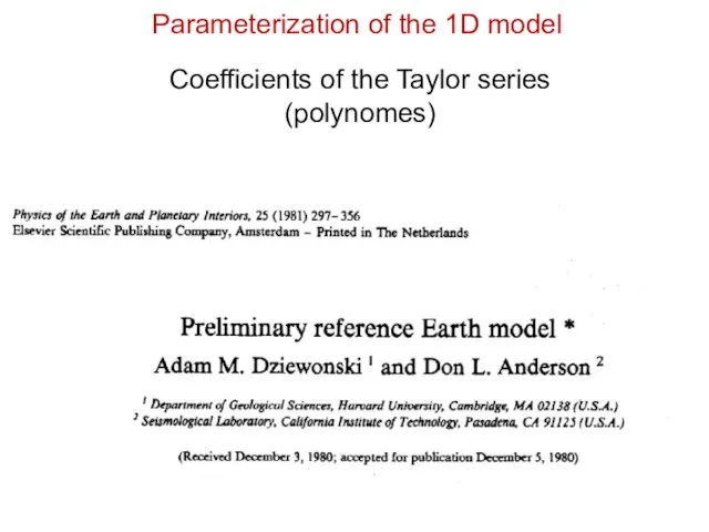
Coefficients of the Taylor series (polynomes)
Parameterization of the 1D model
Coefficients of the Taylor series (polynomes)
Parameterization of the 1D model
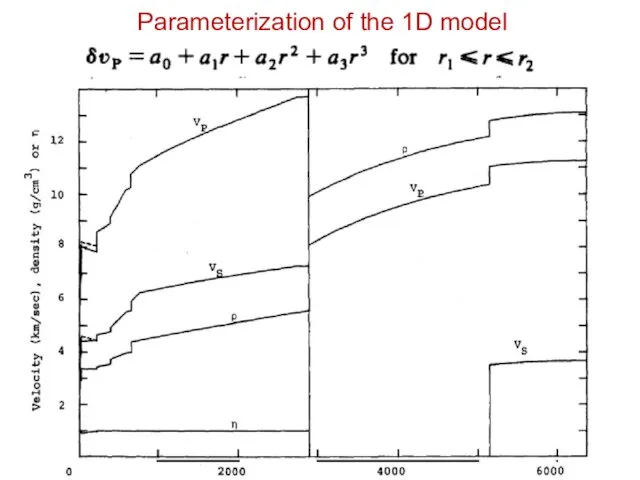
Parameterization of the 1D model
Parameterization of the 1D model
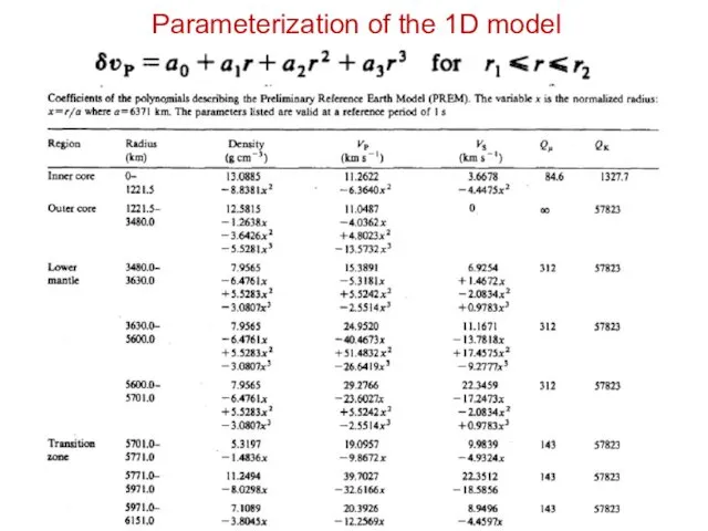
Parameterization of the 1D model
Parameterization of the 1D model
Parameterization of the 1D model
Parameterization of the 1D model
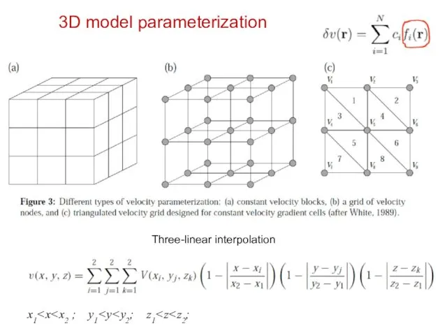
3D model parameterization
Three-linear interpolation
x1
3D model parameterization
Three-linear interpolation
x1
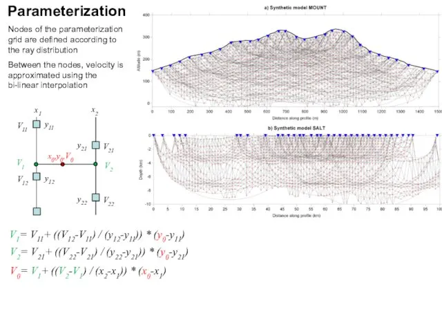
Parameterization
Nodes of the parameterization grid are defined according to the ray
Parameterization
Nodes of the parameterization grid are defined according to the ray
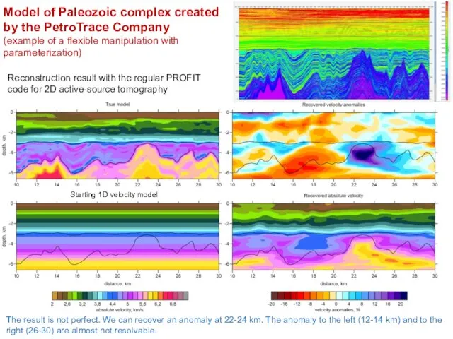
Model of Paleozoic complex created by the PetroTrace Company
(example of a
Model of Paleozoic complex created by the PetroTrace Company
(example of a
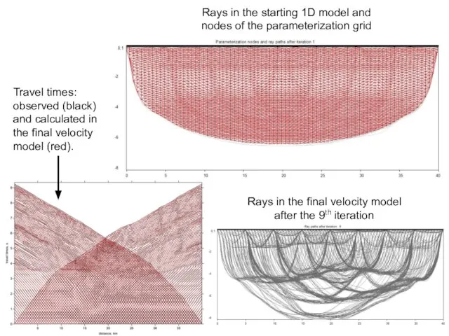
Travel times: observed (black) and calculated in the final velocity model
Travel times: observed (black) and calculated in the final velocity model
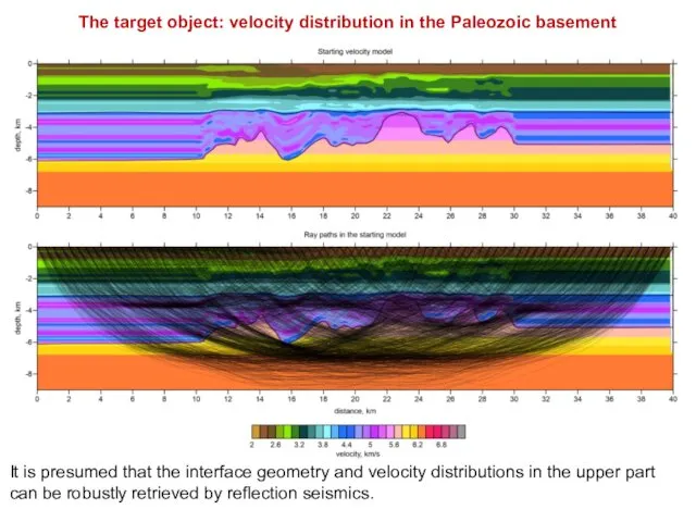
The target object: velocity distribution in the Paleozoic basement
It is presumed
The target object: velocity distribution in the Paleozoic basement
It is presumed
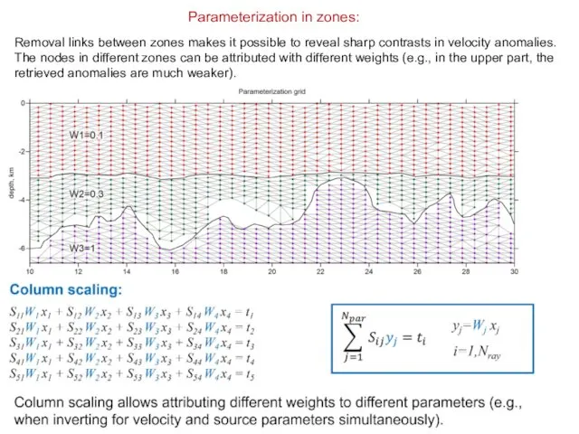
Parameterization in zones:
Removal links between zones makes it possible to reveal
Parameterization in zones:
Removal links between zones makes it possible to reveal
Inversion results with apriori known distributions of velocities in zones 1
Inversion results with apriori known distributions of velocities in zones 1
Inversion results with apriori known distributions of velocities in zones 1
Inversion results with apriori known distributions of velocities in zones 1
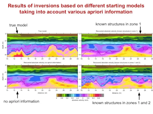
Results of inversions based on different starting models taking into account
Results of inversions based on different starting models taking into account

Regional model parameterization
Cells in the Cartesian coordinates
Performing inversions in several grids
Regional model parameterization
Cells in the Cartesian coordinates
Performing inversions in several grids
Regional model parameterization
Nodes in the Cartesian coordinates
Performing inversions in several grids
Regional model parameterization
Nodes in the Cartesian coordinates
Performing inversions in several grids
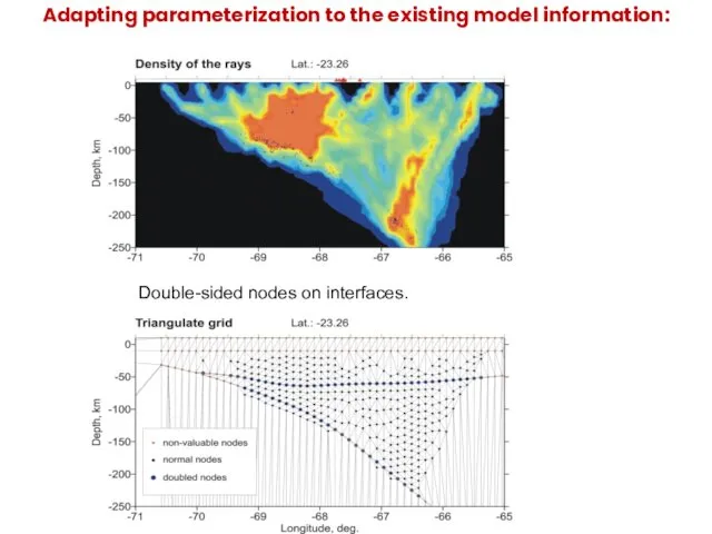
Adapting parameterization to the existing model information:
Double-sided nodes on interfaces.
Adapting parameterization to the existing model information:
Double-sided nodes on interfaces.
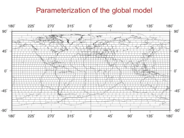
Parameterization of the global model
Parameterization of the global model

Irregular grids (Bijwaard, Spakman et al., 1998)
Irregular grids (Bijwaard, Spakman et al., 1998)
Irregular grid gives a balanced solution depending on the ray coverage
Irregular grid gives a balanced solution depending on the ray coverage
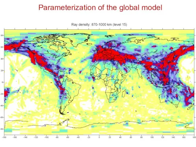
Parameterization of the global model
Parameterization of the global model
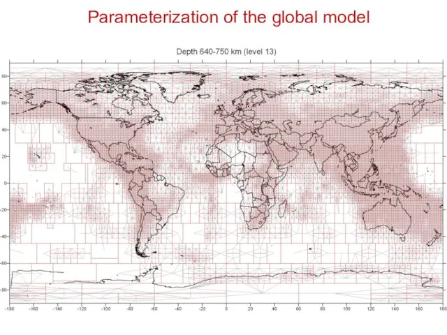
Parameterization of the global model
Parameterization of the global model
Parameterization of the global model
Parameterization of the global model
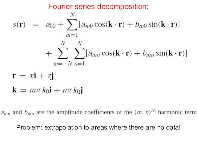
Fourier series decomposition:
Problem: extrapolation to areas where there are no data!
Fourier series decomposition:
Problem: extrapolation to areas where there are no data!
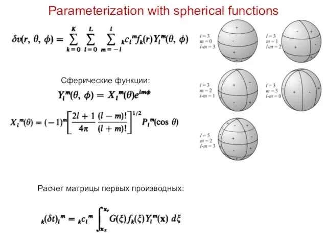
Parameterization with spherical functions
Сферические функции:
Расчет матрицы первых производных:
Parameterization with spherical functions
Сферические функции:
Расчет матрицы первых производных:
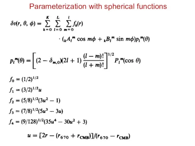
Parameterization with spherical functions
Parameterization with spherical functions
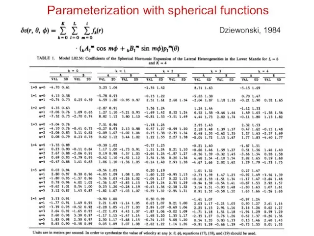
Dziewonski, 1984
Parameterization with spherical functions
Dziewonski, 1984
Parameterization with spherical functions
 Число и цифра 3
 Составление задач
 Презентация по математике "По следам Пифагора" - скачать
  Перемасштабирование каротажных диаграмм
 Матрицы. Виды матриц
 Ещё идут старинные часы (задачи по математике)
 Динамика полета. Системы координат. (Лекция 1)
 Презентация на тему Сумма углов треугольника Решение задач
 Презентация на тему Решение задач с помощью квадратных и рациональных уравнений
  Рационал бөлшектерді қосу және азайту
 Презентация по математике "Виды часов" - скачать бесплатно
 Своя игра. История геометрии
 Умножение и деление на 10
 Прибавление и вычитание числа 2
 Конус
Конус Презентация по математике "Перестановка слагаемых 1 класс" - скачать бесплатно
 Проекции прямой. Начертательная геометрия
 Создание информационной системы анализа математических функций
 10 способов решения квадратных уравнений Работу выполнила учитель математики МБОУ «СОШ №31» г.Энгельса Волосожар М.И.
 Теңдеулер мен теңсіздіктер. Бір айнымалысы бар теңдеулер. Мәндес теңдеулер
 ОГЭ 2018. Модуль Алгебра
 Построение графиков функции
  Решение задач
 Практикум по решению задач №11. (Движение) (профильный уровень)
 Сумма углов треугольника
 «Интересные и быстрые способы и приемы вычислений» Автор: Кузьмина Ирина (8 класс, МОУ «Мисцевская ООШ №2»)
 Виды треугольников. 5 класс
 Положения стереометрической металлографии. (Раздел 1)