- Главная
- Математика
- Time series models. Static models and models with lags
Содержание
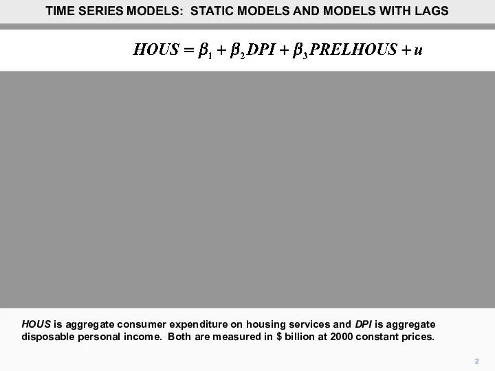
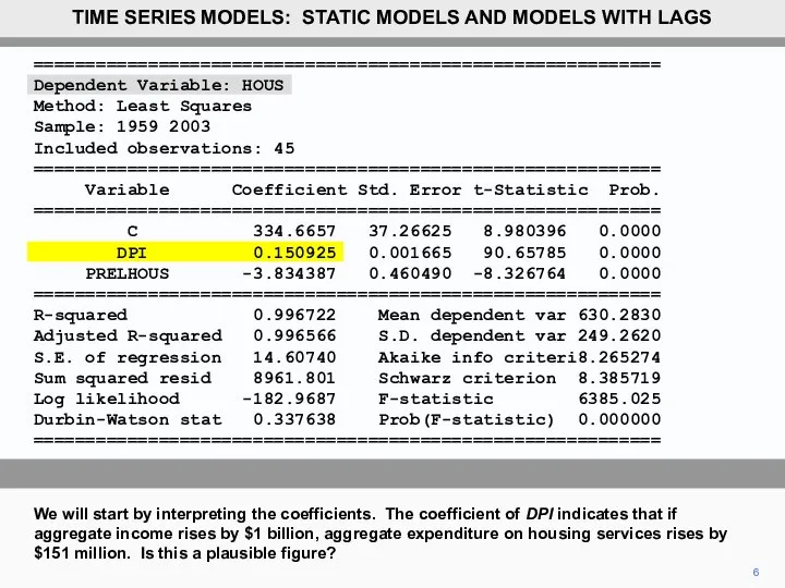
- 2. 2 HOUS is aggregate consumer expenditure on housing services and DPI is aggregate disposable personal income.
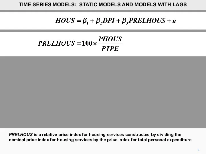
- 3. 3 PRELHOUS is a relative price index for housing services constructed by dividing the nominal price
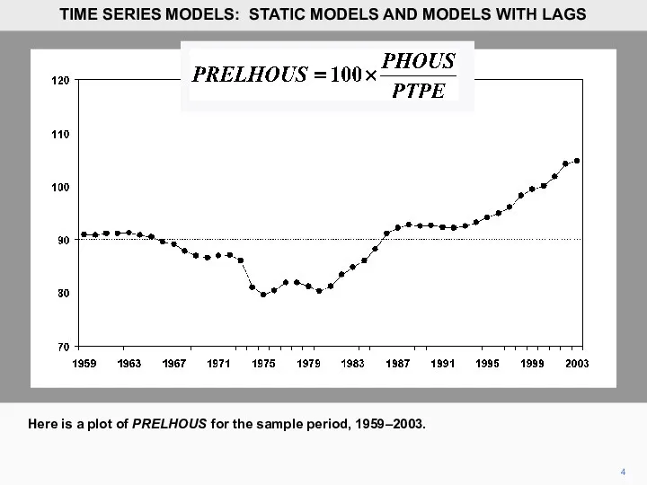
- 4. 4 Here is a plot of PRELHOUS for the sample period, 1959–2003. TIME SERIES MODELS: STATIC
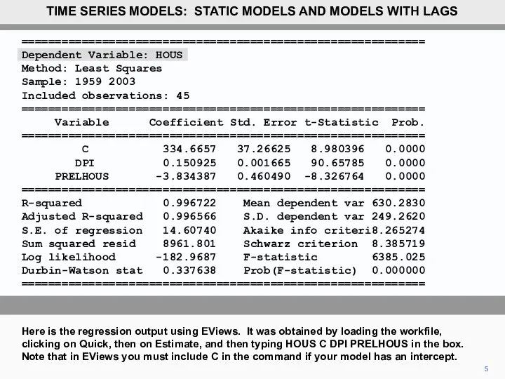
- 5. ============================================================ Dependent Variable: HOUS Method: Least Squares Sample: 1959 2003 Included observations: 45 ============================================================ Variable Coefficient
- 6. ============================================================ Dependent Variable: HOUS Method: Least Squares Sample: 1959 2003 Included observations: 45 ============================================================ Variable Coefficient
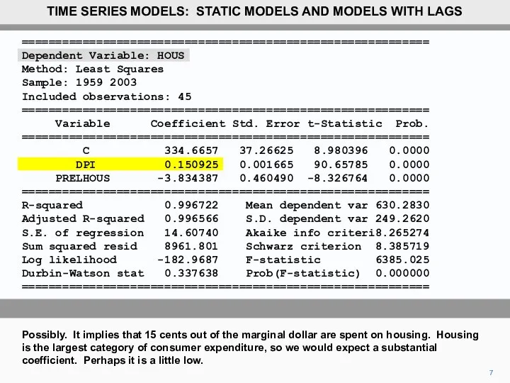
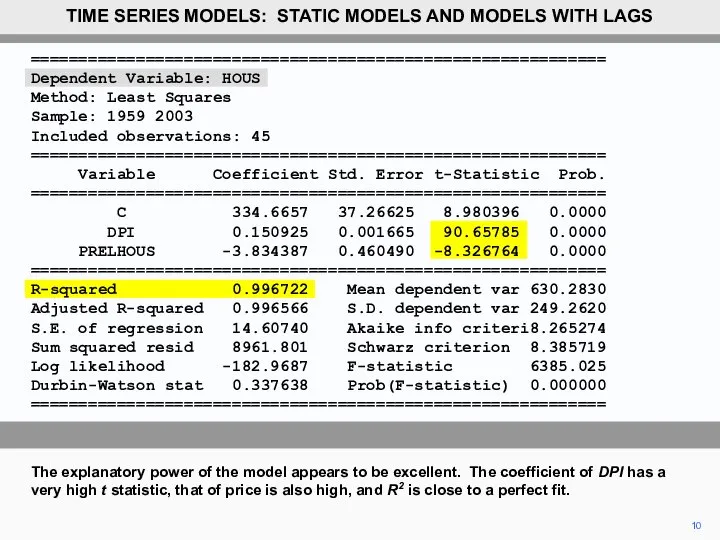
- 7. 7 Possibly. It implies that 15 cents out of the marginal dollar are spent on housing.
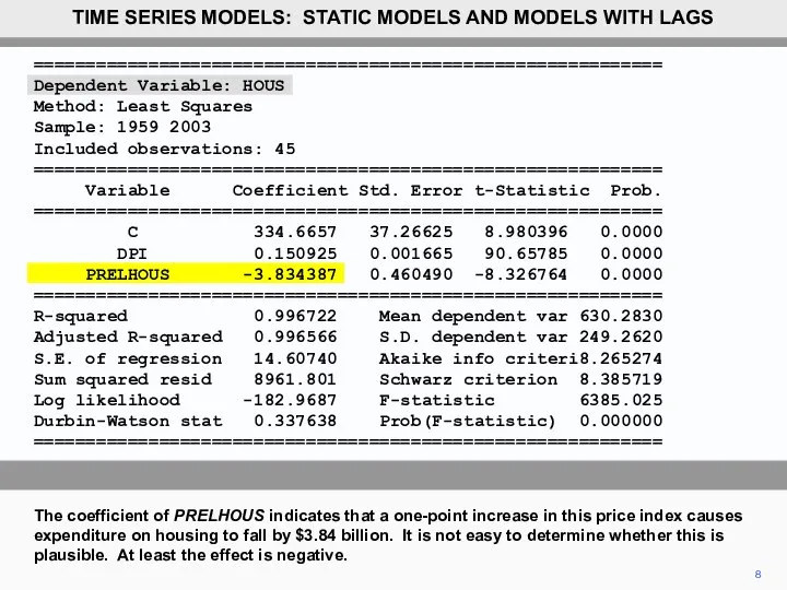
- 8. 8 The coefficient of PRELHOUS indicates that a one-point increase in this price index causes expenditure
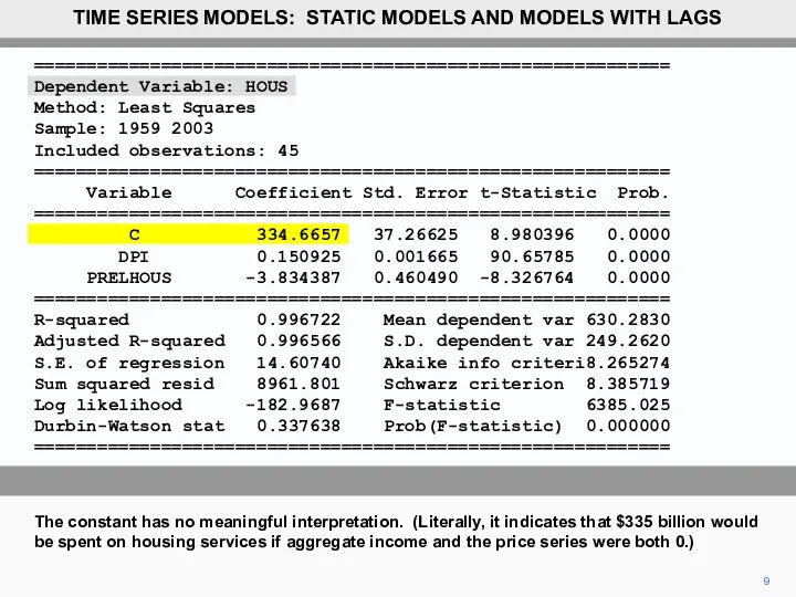
- 9. 9 The constant has no meaningful interpretation. (Literally, it indicates that $335 billion would be spent
- 10. ============================================================ Dependent Variable: HOUS Method: Least Squares Sample: 1959 2003 Included observations: 45 ============================================================ Variable Coefficient
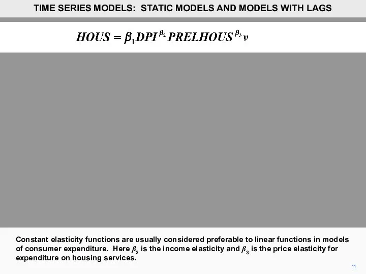
- 11. 11 Constant elasticity functions are usually considered preferable to linear functions in models of consumer expenditure.
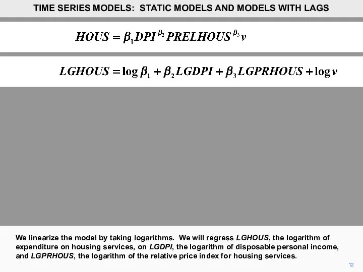
- 12. 12 We linearize the model by taking logarithms. We will regress LGHOUS, the logarithm of expenditure
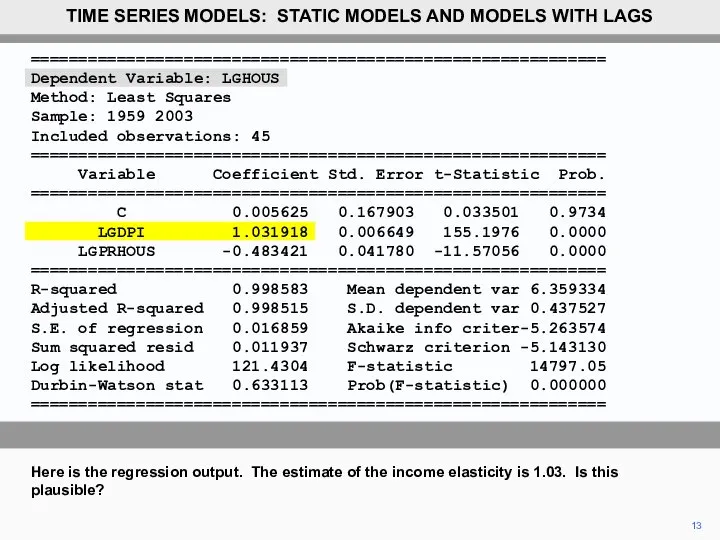
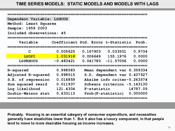
- 13. ============================================================ Dependent Variable: LGHOUS Method: Least Squares Sample: 1959 2003 Included observations: 45 ============================================================ Variable Coefficient
- 14. 14 Probably. Housing is an essential category of consumer expenditure, and necessities generally have elasticities lower
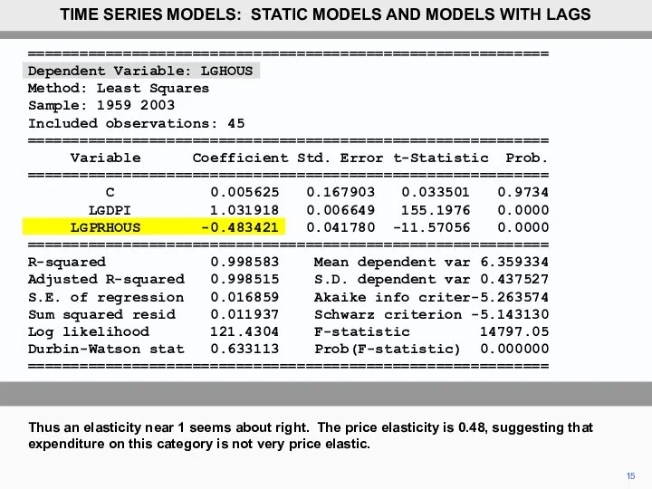
- 15. 15 Thus an elasticity near 1 seems about right. The price elasticity is 0.48, suggesting that
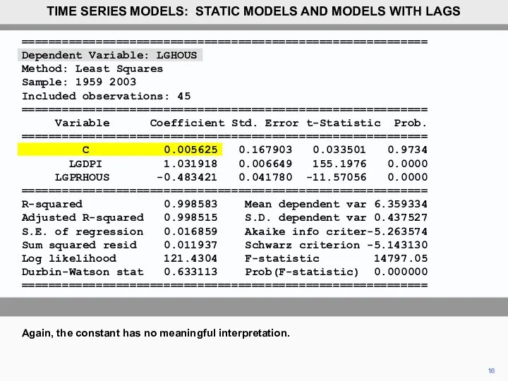
- 16. 16 Again, the constant has no meaningful interpretation. TIME SERIES MODELS: STATIC MODELS AND MODELS WITH
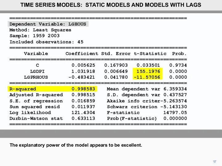
- 17. 17 The explanatory power of the model appears to be excellent. TIME SERIES MODELS: STATIC MODELS
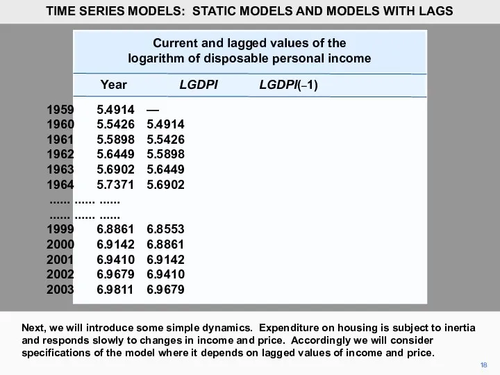
- 18. 18 Next, we will introduce some simple dynamics. Expenditure on housing is subject to inertia and
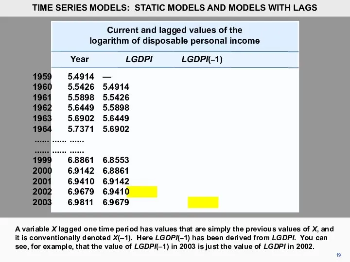
- 19. 19 A variable X lagged one time period has values that are simply the previous values
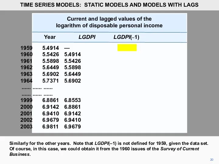
- 20. Current and lagged values of the logarithm of disposable personal income Year LGDPI LGDPI(–1) 1959 5.4914
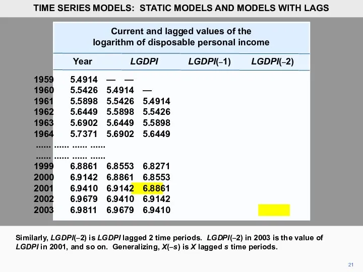
- 21. Current and lagged values of the logarithm of disposable personal income Year LGDPI LGDPI(–1) LGDPI(–2) 1959
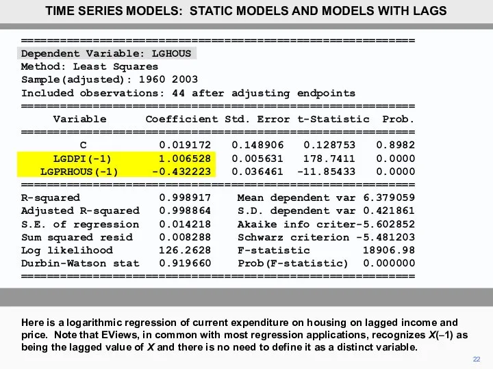
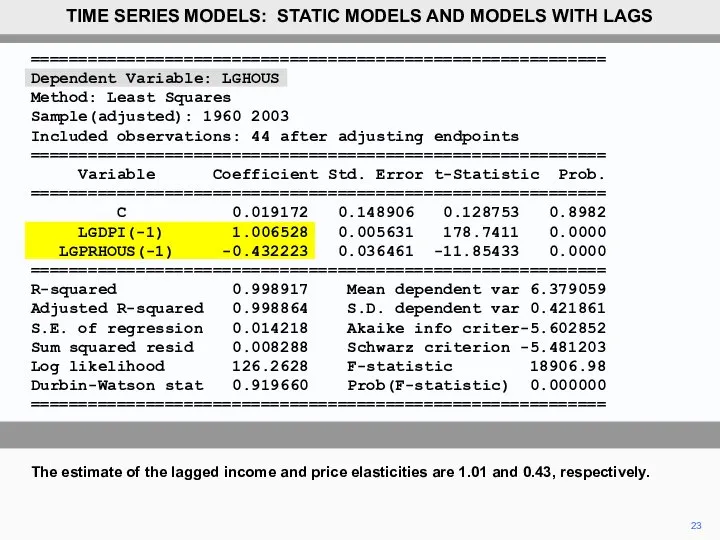
- 22. ============================================================ Dependent Variable: LGHOUS Method: Least Squares Sample(adjusted): 1960 2003 Included observations: 44 after adjusting endpoints
- 23. 23 The estimate of the lagged income and price elasticities are 1.01 and 0.43, respectively. TIME
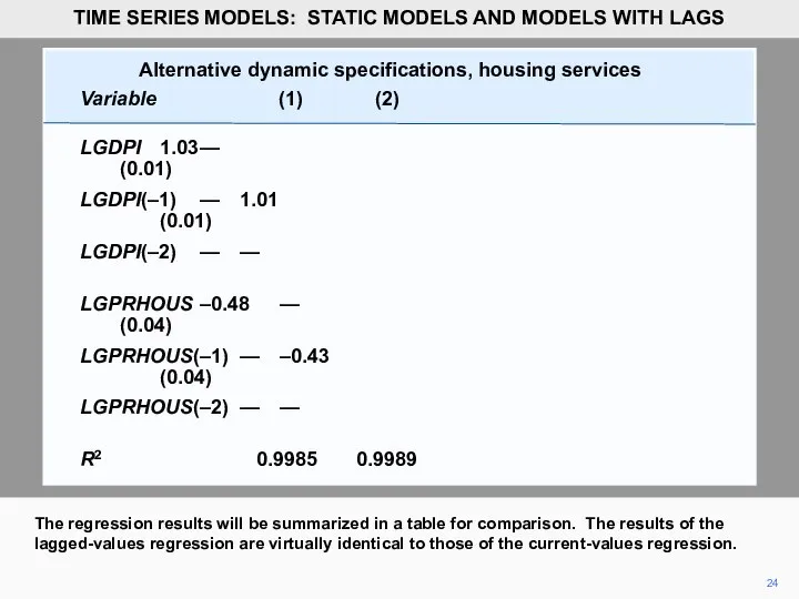
- 24. 24 The regression results will be summarized in a table for comparison. The results of the
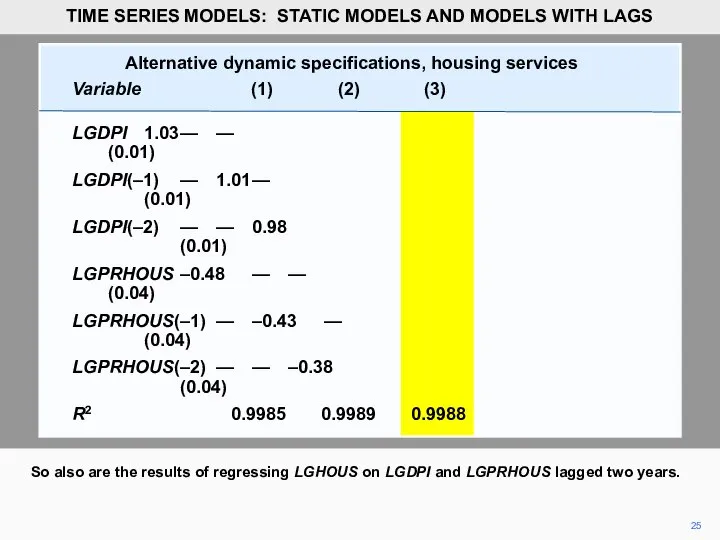
- 25. 25 So also are the results of regressing LGHOUS on LGDPI and LGPRHOUS lagged two years.
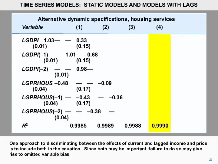
- 26. 26 One approach to discriminating between the effects of current and lagged income and price is
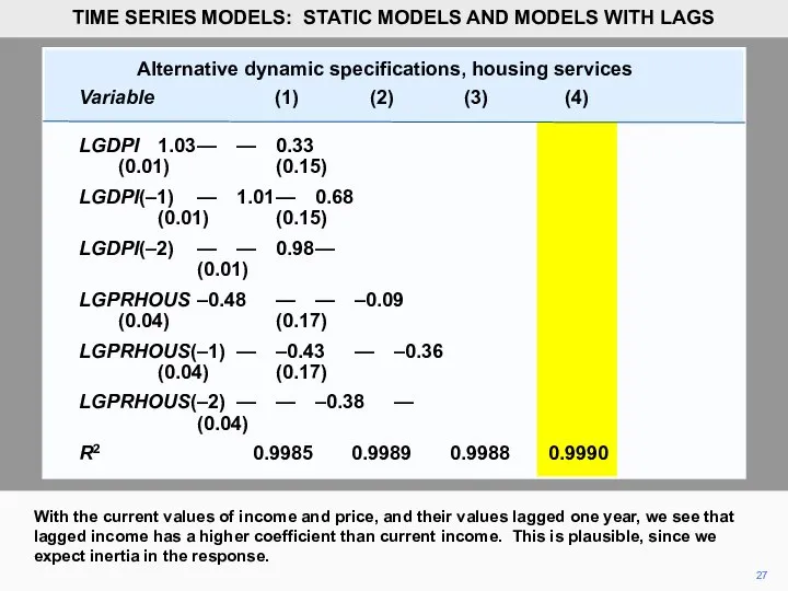
- 27. 27 With the current values of income and price, and their values lagged one year, we
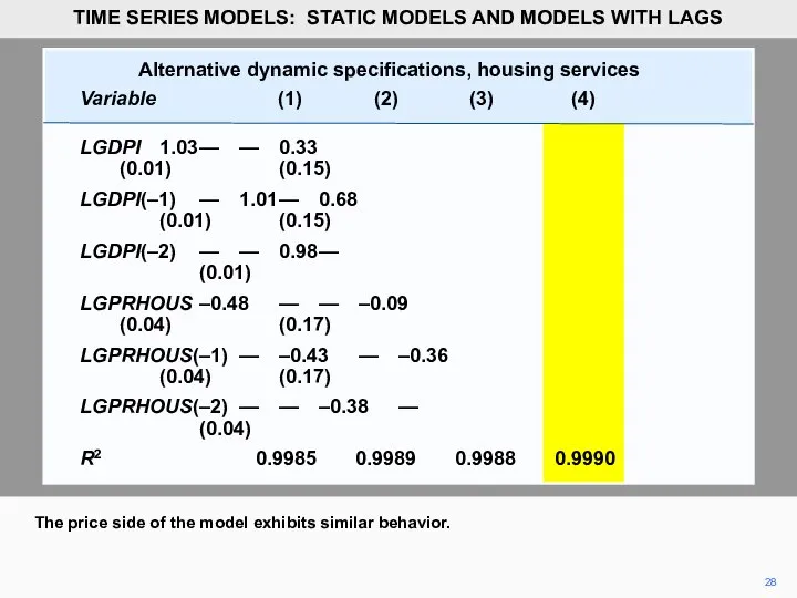
- 28. 28 The price side of the model exhibits similar behavior. TIME SERIES MODELS: STATIC MODELS AND
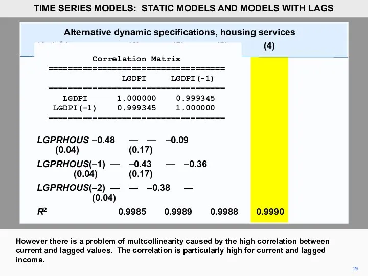
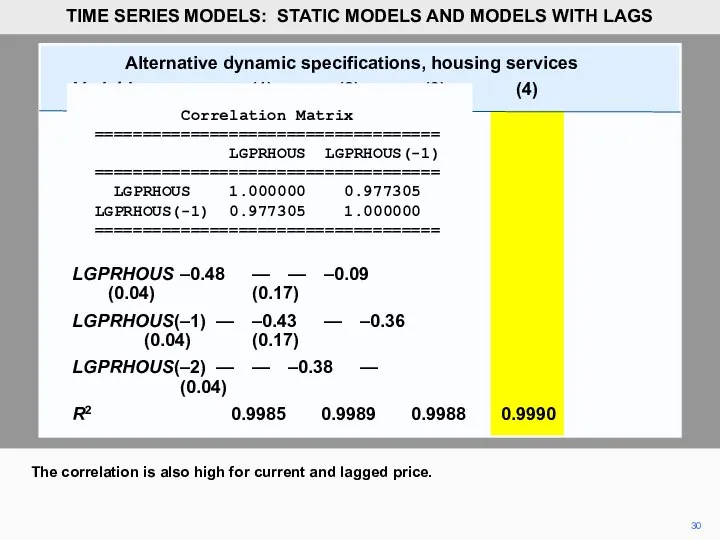
- 29. 29 However there is a problem of multcollinearity caused by the high correlation between current and
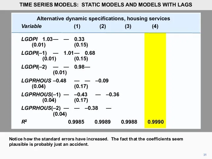
- 30. Alternative dynamic specifications, housing services Variable (1) (2) (3) (4) LGDPI 1.03 — — 0.33 (0.01)
- 31. 31 Notice how the standard errors have increased. The fact that the coefficients seem plausible is
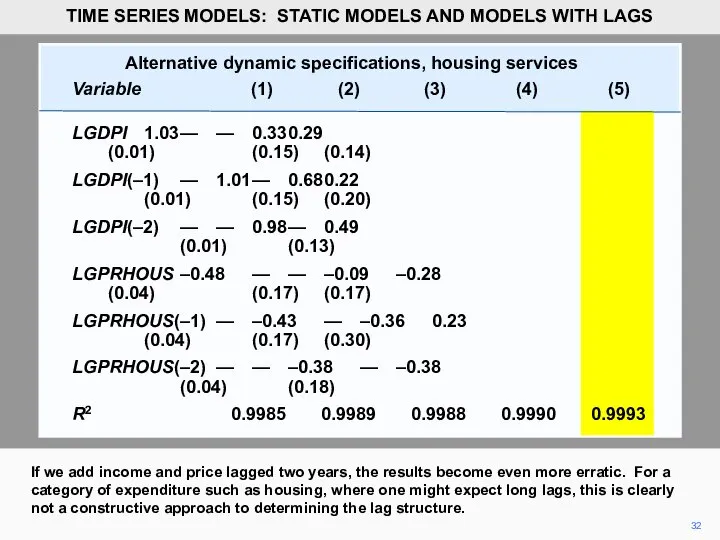
- 32. Alternative dynamic specifications, housing services Variable (1) (2) (3) (4) (5) LGDPI 1.03 — — 0.33
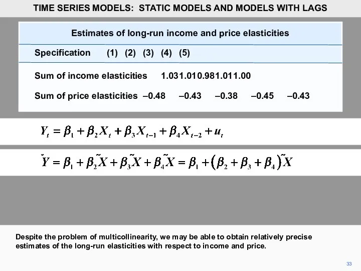
- 33. 33 Despite the problem of multicollinearity, we may be able to obtain relatively precise estimates of
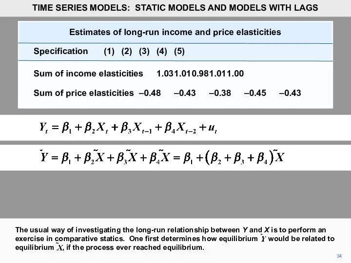
- 34. 34 The usual way of investigating the long-run relationship between Y and X is to perform
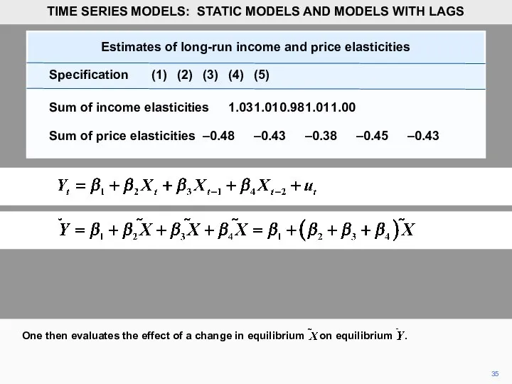
- 35. 35 One then evaluates the effect of a change in equilibrium on equilibrium . TIME SERIES
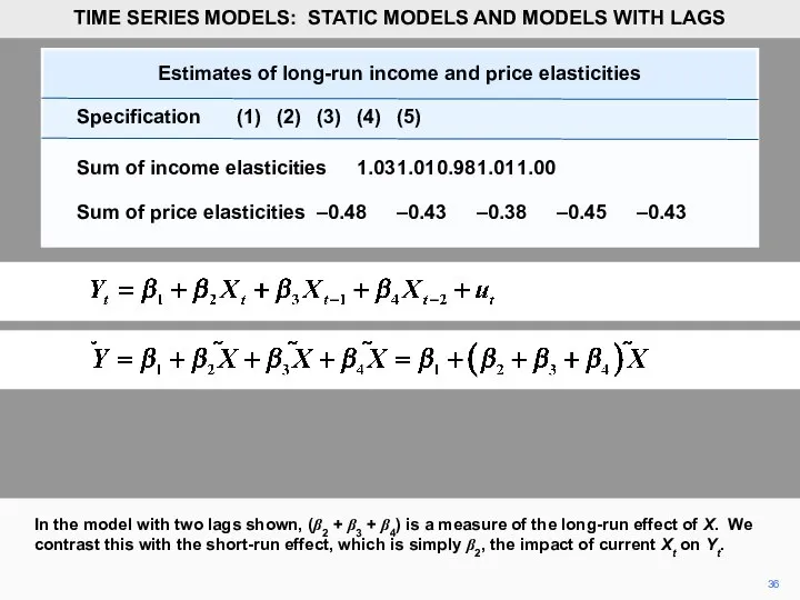
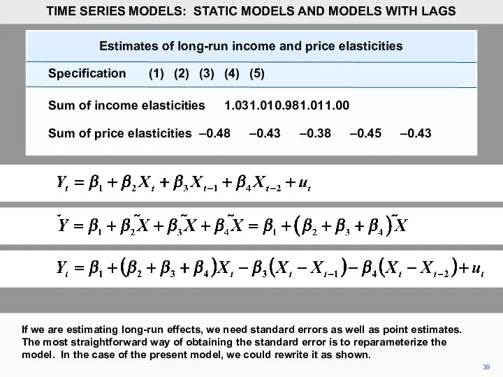
- 36. 36 In the model with two lags shown, (β2 + β3 + β4) is a measure
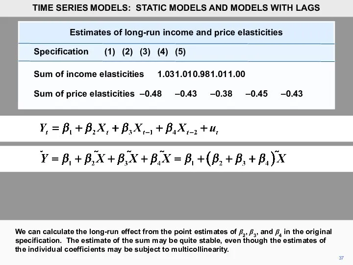
- 37. 37 We can calculate the long-run effect from the point estimates of β2, β3, and β4
- 38. 38 The table presents an example of this. It gives the sum of the income and
- 39. 39 If we are estimating long-run effects, we need standard errors as well as point estimates.
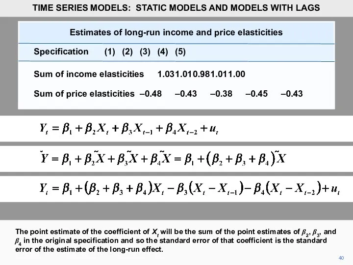
- 40. 40 The point estimate of the coefficient of Xt will be the sum of the point
- 41. 41 Since Xt may well not be highly correlated with (Xt – Xt–1) or (Xt –
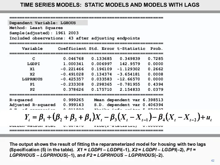
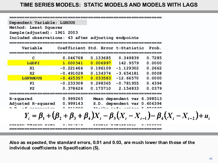
- 42. ============================================================ Dependent Variable: LGHOUS Method: Least Squares Sample(adjusted): 1961 2003 Included observations: 43 after adjusting endpoints
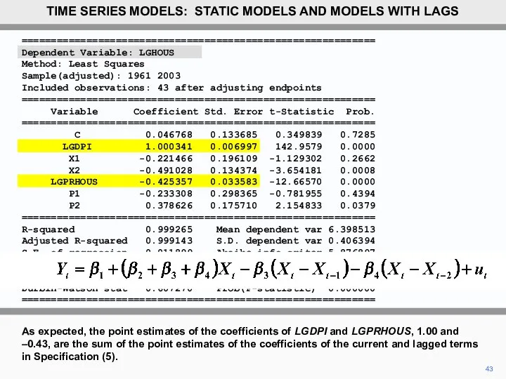
- 43. 43 As expected, the point estimates of the coefficients of LGDPI and LGPRHOUS, 1.00 and –0.43,
- 44. 44 Also as expected, the standard errors, 0.01 and 0.03, are much lower than those of
- 46. Скачать презентацию
2
HOUS is aggregate consumer expenditure on housing services and DPI is
2
HOUS is aggregate consumer expenditure on housing services and DPI is
TIME SERIES MODELS: STATIC MODELS AND MODELS WITH LAGS
3
PRELHOUS is a relative price index for housing services constructed by
3
PRELHOUS is a relative price index for housing services constructed by
TIME SERIES MODELS: STATIC MODELS AND MODELS WITH LAGS
4
Here is a plot of PRELHOUS for the sample period, 1959–2003.
TIME
4
Here is a plot of PRELHOUS for the sample period, 1959–2003.
TIME
============================================================
Dependent Variable: HOUS
Method: Least Squares
Sample: 1959 2003
Included observations:
============================================================
Dependent Variable: HOUS
Method: Least Squares
Sample: 1959 2003
Included observations:
============================================================
Variable Coefficient Std. Error t-Statistic Prob.
============================================================
C 334.6657 37.26625 8.980396 0.0000
DPI 0.150925 0.001665 90.65785 0.0000
PRELHOUS -3.834387 0.460490 -8.326764 0.0000
============================================================
R-squared 0.996722 Mean dependent var 630.2830
Adjusted R-squared 0.996566 S.D. dependent var 249.2620
S.E. of regression 14.60740 Akaike info criteri8.265274
Sum squared resid 8961.801 Schwarz criterion 8.385719
Log likelihood -182.9687 F-statistic 6385.025
Durbin-Watson stat 0.337638 Prob(F-statistic) 0.000000
============================================================
5
Here is the regression output using EViews. It was obtained by loading the workfile, clicking on Quick, then on Estimate, and then typing HOUS C DPI PRELHOUS in the box. Note that in EViews you must include C in the command if your model has an intercept.
TIME SERIES MODELS: STATIC MODELS AND MODELS WITH LAGS
============================================================
Dependent Variable: HOUS
Method: Least Squares
Sample: 1959 2003
Included observations:
============================================================
Dependent Variable: HOUS
Method: Least Squares
Sample: 1959 2003
Included observations:
============================================================
Variable Coefficient Std. Error t-Statistic Prob.
============================================================
C 334.6657 37.26625 8.980396 0.0000
DPI 0.150925 0.001665 90.65785 0.0000
PRELHOUS -3.834387 0.460490 -8.326764 0.0000
============================================================
R-squared 0.996722 Mean dependent var 630.2830
Adjusted R-squared 0.996566 S.D. dependent var 249.2620
S.E. of regression 14.60740 Akaike info criteri8.265274
Sum squared resid 8961.801 Schwarz criterion 8.385719
Log likelihood -182.9687 F-statistic 6385.025
Durbin-Watson stat 0.337638 Prob(F-statistic) 0.000000
============================================================
6
We will start by interpreting the coefficients. The coefficient of DPI indicates that if aggregate income rises by $1 billion, aggregate expenditure on housing services rises by $151 million. Is this a plausible figure?
TIME SERIES MODELS: STATIC MODELS AND MODELS WITH LAGS
7
Possibly. It implies that 15 cents out of the marginal dollar
7
Possibly. It implies that 15 cents out of the marginal dollar
TIME SERIES MODELS: STATIC MODELS AND MODELS WITH LAGS
============================================================
Dependent Variable: HOUS
Method: Least Squares
Sample: 1959 2003
Included observations: 45
============================================================
Variable Coefficient Std. Error t-Statistic Prob.
============================================================
C 334.6657 37.26625 8.980396 0.0000
DPI 0.150925 0.001665 90.65785 0.0000
PRELHOUS -3.834387 0.460490 -8.326764 0.0000
============================================================
R-squared 0.996722 Mean dependent var 630.2830
Adjusted R-squared 0.996566 S.D. dependent var 249.2620
S.E. of regression 14.60740 Akaike info criteri8.265274
Sum squared resid 8961.801 Schwarz criterion 8.385719
Log likelihood -182.9687 F-statistic 6385.025
Durbin-Watson stat 0.337638 Prob(F-statistic) 0.000000
============================================================
8
The coefficient of PRELHOUS indicates that a one-point increase in this
8
The coefficient of PRELHOUS indicates that a one-point increase in this
TIME SERIES MODELS: STATIC MODELS AND MODELS WITH LAGS
============================================================
Dependent Variable: HOUS
Method: Least Squares
Sample: 1959 2003
Included observations: 45
============================================================
Variable Coefficient Std. Error t-Statistic Prob.
============================================================
C 334.6657 37.26625 8.980396 0.0000
DPI 0.150925 0.001665 90.65785 0.0000
PRELHOUS -3.834387 0.460490 -8.326764 0.0000
============================================================
R-squared 0.996722 Mean dependent var 630.2830
Adjusted R-squared 0.996566 S.D. dependent var 249.2620
S.E. of regression 14.60740 Akaike info criteri8.265274
Sum squared resid 8961.801 Schwarz criterion 8.385719
Log likelihood -182.9687 F-statistic 6385.025
Durbin-Watson stat 0.337638 Prob(F-statistic) 0.000000
============================================================
9
The constant has no meaningful interpretation. (Literally, it indicates that $335
9
The constant has no meaningful interpretation. (Literally, it indicates that $335
TIME SERIES MODELS: STATIC MODELS AND MODELS WITH LAGS
============================================================
Dependent Variable: HOUS
Method: Least Squares
Sample: 1959 2003
Included observations: 45
============================================================
Variable Coefficient Std. Error t-Statistic Prob.
============================================================
C 334.6657 37.26625 8.980396 0.0000
DPI 0.150925 0.001665 90.65785 0.0000
PRELHOUS -3.834387 0.460490 -8.326764 0.0000
============================================================
R-squared 0.996722 Mean dependent var 630.2830
Adjusted R-squared 0.996566 S.D. dependent var 249.2620
S.E. of regression 14.60740 Akaike info criteri8.265274
Sum squared resid 8961.801 Schwarz criterion 8.385719
Log likelihood -182.9687 F-statistic 6385.025
Durbin-Watson stat 0.337638 Prob(F-statistic) 0.000000
============================================================
============================================================
Dependent Variable: HOUS
Method: Least Squares
Sample: 1959 2003
Included observations:
============================================================
Dependent Variable: HOUS
Method: Least Squares
Sample: 1959 2003
Included observations:
============================================================
Variable Coefficient Std. Error t-Statistic Prob.
============================================================
C 334.6657 37.26625 8.980396 0.0000
DPI 0.150925 0.001665 90.65785 0.0000
PRELHOUS -3.834387 0.460490 -8.326764 0.0000
============================================================
R-squared 0.996722 Mean dependent var 630.2830
Adjusted R-squared 0.996566 S.D. dependent var 249.2620
S.E. of regression 14.60740 Akaike info criteri8.265274
Sum squared resid 8961.801 Schwarz criterion 8.385719
Log likelihood -182.9687 F-statistic 6385.025
Durbin-Watson stat 0.337638 Prob(F-statistic) 0.000000
============================================================
10
The explanatory power of the model appears to be excellent. The coefficient of DPI has a very high t statistic, that of price is also high, and R2 is close to a perfect fit.
TIME SERIES MODELS: STATIC MODELS AND MODELS WITH LAGS
11
Constant elasticity functions are usually considered preferable to linear functions in
11
Constant elasticity functions are usually considered preferable to linear functions in
TIME SERIES MODELS: STATIC MODELS AND MODELS WITH LAGS
12
We linearize the model by taking logarithms. We will regress LGHOUS,
12
We linearize the model by taking logarithms. We will regress LGHOUS,
TIME SERIES MODELS: STATIC MODELS AND MODELS WITH LAGS
============================================================
Dependent Variable: LGHOUS
Method: Least Squares
Sample: 1959 2003
Included observations:
============================================================
Dependent Variable: LGHOUS
Method: Least Squares
Sample: 1959 2003
Included observations:
============================================================
Variable Coefficient Std. Error t-Statistic Prob.
============================================================
C 0.005625 0.167903 0.033501 0.9734
LGDPI 1.031918 0.006649 155.1976 0.0000
LGPRHOUS -0.483421 0.041780 -11.57056 0.0000
============================================================
R-squared 0.998583 Mean dependent var 6.359334
Adjusted R-squared 0.998515 S.D. dependent var 0.437527
S.E. of regression 0.016859 Akaike info criter-5.263574
Sum squared resid 0.011937 Schwarz criterion -5.143130
Log likelihood 121.4304 F-statistic 14797.05
Durbin-Watson stat 0.633113 Prob(F-statistic) 0.000000
============================================================
13
Here is the regression output. The estimate of the income elasticity is 1.03. Is this plausible?
TIME SERIES MODELS: STATIC MODELS AND MODELS WITH LAGS
14
Probably. Housing is an essential category of consumer expenditure, and necessities
14
Probably. Housing is an essential category of consumer expenditure, and necessities
TIME SERIES MODELS: STATIC MODELS AND MODELS WITH LAGS
============================================================
Dependent Variable: LGHOUS
Method: Least Squares
Sample: 1959 2003
Included observations: 45
============================================================
Variable Coefficient Std. Error t-Statistic Prob.
============================================================
C 0.005625 0.167903 0.033501 0.9734
LGDPI 1.031918 0.006649 155.1976 0.0000
LGPRHOUS -0.483421 0.041780 -11.57056 0.0000
============================================================
R-squared 0.998583 Mean dependent var 6.359334
Adjusted R-squared 0.998515 S.D. dependent var 0.437527
S.E. of regression 0.016859 Akaike info criter-5.263574
Sum squared resid 0.011937 Schwarz criterion -5.143130
Log likelihood 121.4304 F-statistic 14797.05
Durbin-Watson stat 0.633113 Prob(F-statistic) 0.000000
============================================================
15
Thus an elasticity near 1 seems about right. The price elasticity
15
Thus an elasticity near 1 seems about right. The price elasticity
TIME SERIES MODELS: STATIC MODELS AND MODELS WITH LAGS
============================================================
Dependent Variable: LGHOUS
Method: Least Squares
Sample: 1959 2003
Included observations: 45
============================================================
Variable Coefficient Std. Error t-Statistic Prob.
============================================================
C 0.005625 0.167903 0.033501 0.9734
LGDPI 1.031918 0.006649 155.1976 0.0000
LGPRHOUS -0.483421 0.041780 -11.57056 0.0000
============================================================
R-squared 0.998583 Mean dependent var 6.359334
Adjusted R-squared 0.998515 S.D. dependent var 0.437527
S.E. of regression 0.016859 Akaike info criter-5.263574
Sum squared resid 0.011937 Schwarz criterion -5.143130
Log likelihood 121.4304 F-statistic 14797.05
Durbin-Watson stat 0.633113 Prob(F-statistic) 0.000000
============================================================
16
Again, the constant has no meaningful interpretation.
TIME SERIES MODELS: STATIC MODELS
16
Again, the constant has no meaningful interpretation.
TIME SERIES MODELS: STATIC MODELS
============================================================
Dependent Variable: LGHOUS
Method: Least Squares
Sample: 1959 2003
Included observations: 45
============================================================
Variable Coefficient Std. Error t-Statistic Prob.
============================================================
C 0.005625 0.167903 0.033501 0.9734
LGDPI 1.031918 0.006649 155.1976 0.0000
LGPRHOUS -0.483421 0.041780 -11.57056 0.0000
============================================================
R-squared 0.998583 Mean dependent var 6.359334
Adjusted R-squared 0.998515 S.D. dependent var 0.437527
S.E. of regression 0.016859 Akaike info criter-5.263574
Sum squared resid 0.011937 Schwarz criterion -5.143130
Log likelihood 121.4304 F-statistic 14797.05
Durbin-Watson stat 0.633113 Prob(F-statistic) 0.000000
============================================================
17
The explanatory power of the model appears to be excellent.
TIME SERIES
17
The explanatory power of the model appears to be excellent.
TIME SERIES
============================================================
Dependent Variable: LGHOUS
Method: Least Squares
Sample: 1959 2003
Included observations: 45
============================================================
Variable Coefficient Std. Error t-Statistic Prob.
============================================================
C 0.005625 0.167903 0.033501 0.9734
LGDPI 1.031918 0.006649 155.1976 0.0000
LGPRHOUS -0.483421 0.041780 -11.57056 0.0000
============================================================
R-squared 0.998583 Mean dependent var 6.359334
Adjusted R-squared 0.998515 S.D. dependent var 0.437527
S.E. of regression 0.016859 Akaike info criter-5.263574
Sum squared resid 0.011937 Schwarz criterion -5.143130
Log likelihood 121.4304 F-statistic 14797.05
Durbin-Watson stat 0.633113 Prob(F-statistic) 0.000000
============================================================
18
Next, we will introduce some simple dynamics. Expenditure on housing is
18
Next, we will introduce some simple dynamics. Expenditure on housing is
TIME SERIES MODELS: STATIC MODELS AND MODELS WITH LAGS
Current and lagged values of the
logarithm of disposable personal income
Year LGDPI LGDPI(–1)
1959 5.4914 —
1960 5.5426 5.4914
1961 5.5898 5.5426
1962 5.6449 5.5898
1963 5.6902 5.6449
1964 5.7371 5.6902
...... ...... ......
...... ...... ......
1999 6.8861 6.8553
2000 6.9142 6.8861
2001 6.9410 6.9142
2002 6.9679 6.9410
2003 6.9811 6.9679
19
A variable X lagged one time period has values that are
19
A variable X lagged one time period has values that are
TIME SERIES MODELS: STATIC MODELS AND MODELS WITH LAGS
Current and lagged values of the
logarithm of disposable personal income
Year LGDPI LGDPI(–1)
1959 5.4914 —
1960 5.5426 5.4914
1961 5.5898 5.5426
1962 5.6449 5.5898
1963 5.6902 5.6449
1964 5.7371 5.6902
...... ...... ......
...... ...... ......
1999 6.8861 6.8553
2000 6.9142 6.8861
2001 6.9410 6.9142
2002 6.9679 6.9410
2003 6.9811 6.9679
Current and lagged values of the
logarithm of disposable personal income
Year
Current and lagged values of the
logarithm of disposable personal income
Year
1959 5.4914 —
1960 5.5426 5.4914
1961 5.5898 5.5426
1962 5.6449 5.5898
1963 5.6902 5.6449
1964 5.7371 5.6902
...... ...... ......
...... ...... ......
1999 6.8861 6.8553
2000 6.9142 6.8861
2001 6.9410 6.9142
2002 6.9679 6.9410
2003 6.9811 6.9679
20
Similarly for the other years. Note that LGDPI(–1) is not defined for 1959, given the data set. Of course, in this case, we could obtain it from the 1960 issues of the Survey of Current Business.
TIME SERIES MODELS: STATIC MODELS AND MODELS WITH LAGS
Current and lagged values of the
logarithm of disposable personal income
Year
Current and lagged values of the
logarithm of disposable personal income
Year
1959 5.4914 — —
1960 5.5426 5.4914 —
1961 5.5898 5.5426 5.4914
1962 5.6449 5.5898 5.5426
1963 5.6902 5.6449 5.5898
1964 5.7371 5.6902 5.6449
...... ...... ...... ......
...... ...... ...... ......
1999 6.8861 6.8553 6.8271
2000 6.9142 6.8861 6.8553
2001 6.9410 6.9142 6.8861
2002 6.9679 6.9410 6.9142
2003 6.9811 6.9679 6.9410
21
Similarly, LGDPI(–2) is LGDPI lagged 2 time periods. LGDPI(–2) in 2003 is the value of LGDPI in 2001, and so on. Generalizing, X(–s) is X lagged s time periods.
TIME SERIES MODELS: STATIC MODELS AND MODELS WITH LAGS
============================================================
Dependent Variable: LGHOUS
Method: Least Squares
Sample(adjusted): 1960 2003
Included observations:
============================================================
Dependent Variable: LGHOUS
Method: Least Squares
Sample(adjusted): 1960 2003
Included observations:
============================================================
Variable Coefficient Std. Error t-Statistic Prob.
============================================================
C 0.019172 0.148906 0.128753 0.8982
LGDPI(-1) 1.006528 0.005631 178.7411 0.0000
LGPRHOUS(-1) -0.432223 0.036461 -11.85433 0.0000
============================================================
R-squared 0.998917 Mean dependent var 6.379059
Adjusted R-squared 0.998864 S.D. dependent var 0.421861
S.E. of regression 0.014218 Akaike info criter-5.602852
Sum squared resid 0.008288 Schwarz criterion -5.481203
Log likelihood 126.2628 F-statistic 18906.98
Durbin-Watson stat 0.919660 Prob(F-statistic) 0.000000
============================================================
22
Here is a logarithmic regression of current expenditure on housing on lagged income and price. Note that EViews, in common with most regression applications, recognizes X(–1) as being the lagged value of X and there is no need to define it as a distinct variable.
TIME SERIES MODELS: STATIC MODELS AND MODELS WITH LAGS
23
The estimate of the lagged income and price elasticities are 1.01
23
The estimate of the lagged income and price elasticities are 1.01
TIME SERIES MODELS: STATIC MODELS AND MODELS WITH LAGS
============================================================
Dependent Variable: LGHOUS
Method: Least Squares
Sample(adjusted): 1960 2003
Included observations: 44 after adjusting endpoints
============================================================
Variable Coefficient Std. Error t-Statistic Prob.
============================================================
C 0.019172 0.148906 0.128753 0.8982
LGDPI(-1) 1.006528 0.005631 178.7411 0.0000
LGPRHOUS(-1) -0.432223 0.036461 -11.85433 0.0000
============================================================
R-squared 0.998917 Mean dependent var 6.379059
Adjusted R-squared 0.998864 S.D. dependent var 0.421861
S.E. of regression 0.014218 Akaike info criter-5.602852
Sum squared resid 0.008288 Schwarz criterion -5.481203
Log likelihood 126.2628 F-statistic 18906.98
Durbin-Watson stat 0.919660 Prob(F-statistic) 0.000000
============================================================
24
The regression results will be summarized in a table for comparison.
24
The regression results will be summarized in a table for comparison.
TIME SERIES MODELS: STATIC MODELS AND MODELS WITH LAGS
Alternative dynamic specifications, housing services
Variable (1) (2)
LGDPI 1.03 —
(0.01)
LGDPI(–1) — 1.01
(0.01)
LGDPI(–2) — —
LGPRHOUS –0.48 —
(0.04)
LGPRHOUS(–1) — –0.43
(0.04)
LGPRHOUS(–2) — —
R2 0.9985 0.9989
25
So also are the results of regressing LGHOUS on LGDPI and
25
So also are the results of regressing LGHOUS on LGDPI and
TIME SERIES MODELS: STATIC MODELS AND MODELS WITH LAGS
Alternative dynamic specifications, housing services
Variable (1) (2) (3)
LGDPI 1.03 — —
(0.01)
LGDPI(–1) — 1.01 —
(0.01)
LGDPI(–2) — — 0.98
(0.01)
LGPRHOUS –0.48 — —
(0.04)
LGPRHOUS(–1) — –0.43 —
(0.04)
LGPRHOUS(–2) — — –0.38
(0.04)
R2 0.9985 0.9989 0.9988
26
One approach to discriminating between the effects of current and lagged
26
One approach to discriminating between the effects of current and lagged
TIME SERIES MODELS: STATIC MODELS AND MODELS WITH LAGS
Alternative dynamic specifications, housing services
Variable (1) (2) (3) (4)
LGDPI 1.03 — — 0.33
(0.01) (0.15)
LGDPI(–1) — 1.01 — 0.68
(0.01) (0.15)
LGDPI(–2) — — 0.98 —
(0.01)
LGPRHOUS –0.48 — — –0.09
(0.04) (0.17)
LGPRHOUS(–1) — –0.43 — –0.36
(0.04) (0.17)
LGPRHOUS(–2) — — –0.38 —
(0.04)
R2 0.9985 0.9989 0.9988 0.9990
27
With the current values of income and price, and their values
27
With the current values of income and price, and their values
TIME SERIES MODELS: STATIC MODELS AND MODELS WITH LAGS
Alternative dynamic specifications, housing services
Variable (1) (2) (3) (4)
LGDPI 1.03 — — 0.33
(0.01) (0.15)
LGDPI(–1) — 1.01 — 0.68
(0.01) (0.15)
LGDPI(–2) — — 0.98 —
(0.01)
LGPRHOUS –0.48 — — –0.09
(0.04) (0.17)
LGPRHOUS(–1) — –0.43 — –0.36
(0.04) (0.17)
LGPRHOUS(–2) — — –0.38 —
(0.04)
R2 0.9985 0.9989 0.9988 0.9990
28
The price side of the model exhibits similar behavior.
TIME SERIES MODELS:
28
The price side of the model exhibits similar behavior.
TIME SERIES MODELS:
Alternative dynamic specifications, housing services
Variable (1) (2) (3) (4)
LGDPI 1.03 — — 0.33
(0.01) (0.15)
LGDPI(–1) — 1.01 — 0.68
(0.01) (0.15)
LGDPI(–2) — — 0.98 —
(0.01)
LGPRHOUS –0.48 — — –0.09
(0.04) (0.17)
LGPRHOUS(–1) — –0.43 — –0.36
(0.04) (0.17)
LGPRHOUS(–2) — — –0.38 —
(0.04)
R2 0.9985 0.9989 0.9988 0.9990
29
However there is a problem of multcollinearity caused by the high
29
However there is a problem of multcollinearity caused by the high
TIME SERIES MODELS: STATIC MODELS AND MODELS WITH LAGS
Alternative dynamic specifications, housing services
Variable (1) (2) (3) (4)
LGDPI 1.03 — — 0.33
(0.01) (0.15)
LGDPI(–1) — 1.01 — 0.68
(0.01) (0.15)
LGDPI(–2) — — 0.98 —
(0.01)
LGPRHOUS –0.48 — — –0.09
(0.04) (0.17)
LGPRHOUS(–1) — –0.43 — –0.36
(0.04) (0.17)
LGPRHOUS(–2) — — –0.38 —
(0.04)
R2 0.9985 0.9989 0.9988 0.9990
Correlation Matrix
====================================
LGDPI LGDPI(-1)
====================================
LGDPI 1.000000 0.999345
LGDPI(-1) 0.999345 1.000000
====================================
Alternative dynamic specifications, housing services
Variable (1) (2) (3) (4)
LGDPI 1.03 — — 0.33
(0.01) (0.15)
LGDPI(–1) — 1.01 — 0.68
(0.01) (0.15)
LGDPI(–2) — — 0.98 —
(0.01)
LGPRHOUS –0.48 — — –0.09
(0.04) (0.17)
LGPRHOUS(–1) — –0.43 — –0.36
(0.04) (0.17)
LGPRHOUS(–2) — — –0.38 —
(0.04)
R2 0.9985
Variable (1) (2) (3) (4)
LGDPI 1.03 — — 0.33
(0.01) (0.15)
LGDPI(–1) — 1.01 — 0.68
(0.01) (0.15)
LGDPI(–2) — — 0.98 —
(0.01)
LGPRHOUS –0.48 — — –0.09
(0.04) (0.17)
LGPRHOUS(–1) — –0.43 — –0.36
(0.04) (0.17)
LGPRHOUS(–2) — — –0.38 —
(0.04)
R2 0.9985
30
Correlation Matrix
====================================
LGPRHOUS LGPRHOUS(-1)
====================================
LGPRHOUS 1.000000 0.977305
LGPRHOUS(-1) 0.977305 1.000000
====================================
The correlation is also high for current and lagged price.
TIME SERIES MODELS: STATIC MODELS AND MODELS WITH LAGS
31
Notice how the standard errors have increased. The fact that the
31
Notice how the standard errors have increased. The fact that the
TIME SERIES MODELS: STATIC MODELS AND MODELS WITH LAGS
Alternative dynamic specifications, housing services
Variable (1) (2) (3) (4)
LGDPI 1.03 — — 0.33
(0.01) (0.15)
LGDPI(–1) — 1.01 — 0.68
(0.01) (0.15)
LGDPI(–2) — — 0.98 —
(0.01)
LGPRHOUS –0.48 — — –0.09
(0.04) (0.17)
LGPRHOUS(–1) — –0.43 — –0.36
(0.04) (0.17)
LGPRHOUS(–2) — — –0.38 —
(0.04)
R2 0.9985 0.9989 0.9988 0.9990
Alternative dynamic specifications, housing services
Variable (1) (2) (3) (4) (5)
LGDPI 1.03 — — 0.33 0.29
(0.01) (0.15) (0.14)
LGDPI(–1) — 1.01 — 0.68 0.22
(0.01) (0.15) (0.20)
LGDPI(–2) — — 0.98 — 0.49
(0.01) (0.13)
LGPRHOUS –0.48 — — –0.09 –0.28
(0.04) (0.17) (0.17)
LGPRHOUS(–1) — –0.43 — –0.36 0.23
(0.04) (0.17) (0.30)
LGPRHOUS(–2) — — –0.38 — –0.38
(0.04) (0.18)
R2 0.9985
32
If we add income and price lagged two years, the results become even more erratic. For a category of expenditure such as housing, where one might expect long lags, this is clearly not a constructive approach to determining the lag structure.
TIME SERIES MODELS: STATIC MODELS AND MODELS WITH LAGS
33
Despite the problem of multicollinearity, we may be able to obtain
33
Despite the problem of multicollinearity, we may be able to obtain
TIME SERIES MODELS: STATIC MODELS AND MODELS WITH LAGS
Estimates of long-run income and price elasticities
Specification (1) (2) (3) (4) (5)
Sum of income elasticities 1.03 1.01 0.98 1.01 1.00
Sum of price elasticities –0.48 –0.43 –0.38 –0.45 –0.43
34
The usual way of investigating the long-run relationship between Y and
34
The usual way of investigating the long-run relationship between Y and
TIME SERIES MODELS: STATIC MODELS AND MODELS WITH LAGS
Estimates of long-run income and price elasticities
Specification (1) (2) (3) (4) (5)
Sum of income elasticities 1.03 1.01 0.98 1.01 1.00
Sum of price elasticities –0.48 –0.43 –0.38 –0.45 –0.43
35
One then evaluates the effect of a change in equilibrium on
35
One then evaluates the effect of a change in equilibrium on
TIME SERIES MODELS: STATIC MODELS AND MODELS WITH LAGS
Estimates of long-run income and price elasticities
Specification (1) (2) (3) (4) (5)
Sum of income elasticities 1.03 1.01 0.98 1.01 1.00
Sum of price elasticities –0.48 –0.43 –0.38 –0.45 –0.43
36
In the model with two lags shown, (β2 + β3 +
36
In the model with two lags shown, (β2 + β3 +
TIME SERIES MODELS: STATIC MODELS AND MODELS WITH LAGS
Estimates of long-run income and price elasticities
Specification (1) (2) (3) (4) (5)
Sum of income elasticities 1.03 1.01 0.98 1.01 1.00
Sum of price elasticities –0.48 –0.43 –0.38 –0.45 –0.43
37
We can calculate the long-run effect from the point estimates of
37
We can calculate the long-run effect from the point estimates of
TIME SERIES MODELS: STATIC MODELS AND MODELS WITH LAGS
Estimates of long-run income and price elasticities
Specification (1) (2) (3) (4) (5)
Sum of income elasticities 1.03 1.01 0.98 1.01 1.00
Sum of price elasticities –0.48 –0.43 –0.38 –0.45 –0.43
38
The table presents an example of this. It gives the sum
38
The table presents an example of this. It gives the sum
TIME SERIES MODELS: STATIC MODELS AND MODELS WITH LAGS
Estimates of long-run income and price elasticities
Specification (1) (2) (3) (4) (5)
Sum of income elasticities 1.03 1.01 0.98 1.01 1.00
Sum of price elasticities –0.48 –0.43 –0.38 –0.45 –0.43
39
If we are estimating long-run effects, we need standard errors as
39
If we are estimating long-run effects, we need standard errors as
TIME SERIES MODELS: STATIC MODELS AND MODELS WITH LAGS
Estimates of long-run income and price elasticities
Specification (1) (2) (3) (4) (5)
Sum of income elasticities 1.03 1.01 0.98 1.01 1.00
Sum of price elasticities –0.48 –0.43 –0.38 –0.45 –0.43
40
The point estimate of the coefficient of Xt will be the
40
The point estimate of the coefficient of Xt will be the
TIME SERIES MODELS: STATIC MODELS AND MODELS WITH LAGS
Estimates of long-run income and price elasticities
Specification (1) (2) (3) (4) (5)
Sum of income elasticities 1.03 1.01 0.98 1.01 1.00
Sum of price elasticities –0.48 –0.43 –0.38 –0.45 –0.43
41
Since Xt may well not be highly correlated with (Xt –
41
Since Xt may well not be highly correlated with (Xt –
TIME SERIES MODELS: STATIC MODELS AND MODELS WITH LAGS
Estimates of long-run income and price elasticities
Specification (1) (2) (3) (4) (5)
Sum of income elasticities 1.03 1.01 0.98 1.01 1.00
Sum of price elasticities –0.48 –0.43 –0.38 –0.45 –0.43
============================================================
Dependent Variable: LGHOUS
Method: Least Squares
Sample(adjusted): 1961 2003
Included observations:
============================================================
Dependent Variable: LGHOUS
Method: Least Squares
Sample(adjusted): 1961 2003
Included observations:
============================================================
Variable Coefficient Std. Error t-Statistic Prob.
============================================================
C 0.046768 0.133685 0.349839 0.7285
LGDPI 1.000341 0.006997 142.9579 0.0000
X1 -0.221466 0.196109 -1.129302 0.2662
X2 -0.491028 0.134374 -3.654181 0.0008
LGPRHOUS -0.425357 0.033583 -12.66570 0.0000
P1 -0.233308 0.298365 -0.781955 0.4394
P2 0.378626 0.175710 2.154833 0.0379
============================================================
R-squared 0.999265 Mean dependent var 6.398513
Adjusted R-squared 0.999143 S.D. dependent var 0.406394
S.E. of regression 0.011899 Akaike info criter-5.876897
Sum squared resid 0.005097 Schwarz criterion -5.590190
Log likelihood 133.3533 F-statistic 8159.882
Durbin-Watson stat 0.607270 Prob(F-statistic) 0.000000
============================================================
42
The output shows the result of fitting the reparameterized model for housing with two lags (Specification (5) in the table). X1 = LGDPI – LGDPI(–1), X2 = LGDPI – LGDPI(–2), P1 = LGPRHOUS – LGPRHOUS(–1), and P2 = LGPRHOUS – LGPRHOUS(–2).
TIME SERIES MODELS: STATIC MODELS AND MODELS WITH LAGS
43
As expected, the point estimates of the coefficients of LGDPI and
43
As expected, the point estimates of the coefficients of LGDPI and
–0.43, are the sum of the point estimates of the coefficients of the current and lagged terms in Specification (5).
TIME SERIES MODELS: STATIC MODELS AND MODELS WITH LAGS
============================================================
Dependent Variable: LGHOUS
Method: Least Squares
Sample(adjusted): 1961 2003
Included observations: 43 after adjusting endpoints
============================================================
Variable Coefficient Std. Error t-Statistic Prob.
============================================================
C 0.046768 0.133685 0.349839 0.7285
LGDPI 1.000341 0.006997 142.9579 0.0000
X1 -0.221466 0.196109 -1.129302 0.2662
X2 -0.491028 0.134374 -3.654181 0.0008
LGPRHOUS -0.425357 0.033583 -12.66570 0.0000
P1 -0.233308 0.298365 -0.781955 0.4394
P2 0.378626 0.175710 2.154833 0.0379
============================================================
R-squared 0.999265 Mean dependent var 6.398513
Adjusted R-squared 0.999143 S.D. dependent var 0.406394
S.E. of regression 0.011899 Akaike info criter-5.876897
Sum squared resid 0.005097 Schwarz criterion -5.590190
Log likelihood 133.3533 F-statistic 8159.882
Durbin-Watson stat 0.607270 Prob(F-statistic) 0.000000
============================================================
44
Also as expected, the standard errors, 0.01 and 0.03, are much
44
Also as expected, the standard errors, 0.01 and 0.03, are much
TIME SERIES MODELS: STATIC MODELS AND MODELS WITH LAGS
============================================================
Dependent Variable: LGHOUS
Method: Least Squares
Sample(adjusted): 1961 2003
Included observations: 43 after adjusting endpoints
============================================================
Variable Coefficient Std. Error t-Statistic Prob.
============================================================
C 0.046768 0.133685 0.349839 0.7285
LGDPI 1.000341 0.006997 142.9579 0.0000
X1 -0.221466 0.196109 -1.129302 0.2662
X2 -0.491028 0.134374 -3.654181 0.0008
LGPRHOUS -0.425357 0.033583 -12.66570 0.0000
P1 -0.233308 0.298365 -0.781955 0.4394
P2 0.378626 0.175710 2.154833 0.0379
============================================================
R-squared 0.999265 Mean dependent var 6.398513
Adjusted R-squared 0.999143 S.D. dependent var 0.406394
S.E. of regression 0.011899 Akaike info criter-5.876897
Sum squared resid 0.005097 Schwarz criterion -5.590190
Log likelihood 133.3533 F-statistic 8159.882
Durbin-Watson stat 0.607270 Prob(F-statistic) 0.000000
============================================================