- Aggregate Demand I. Building the IS–LM Model

Содержание
- 2. 11-1 The Goods Market and the IS Curve 11-2 The Money Market and the LM Curve
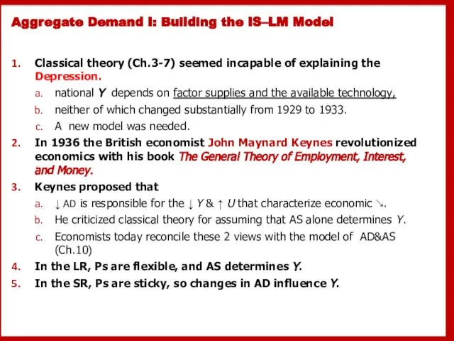
- 3. Aggregate Demand I: Building the IS–LM Model Classical theory (Ch.3-7) seemed incapable of explaining the Depression.
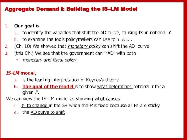
- 4. Aggregate Demand I: Building the IS–LM Model Our goal is to identify the variables that shift
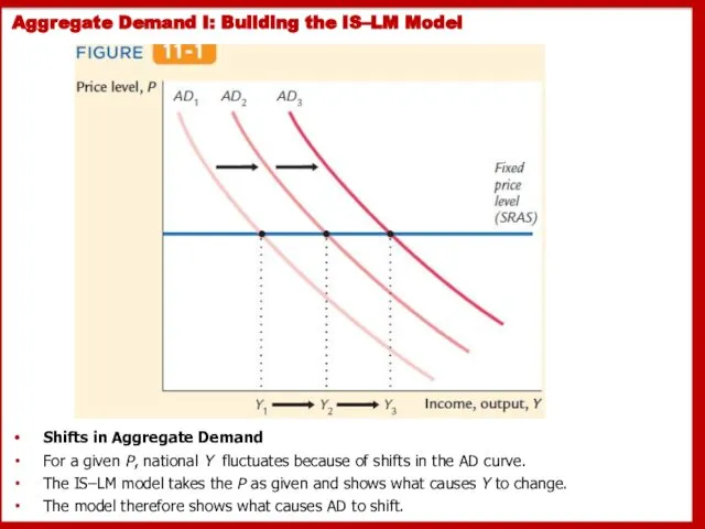
- 5. Aggregate Demand I: Building the IS–LM Model Shifts in Aggregate Demand For a given P, national
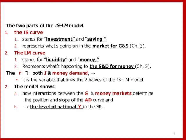
- 6. The two parts of the IS–LM model the IS curve stands for “investment’’ and “saving,’’ represents
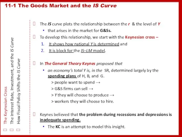
- 7. The IS curve plots the relationship between the r & the level of Y that arises
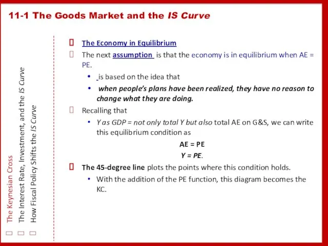
- 8. 11-1 The Goods Market and the IS Curve The Keynesian Cross The Interest Rate, Investment, and
- 9. 11-1 The Goods Market and the IS Curve The Keynesian Cross The Interest Rate, Investment, and
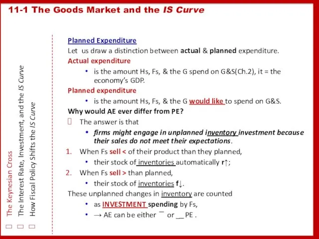
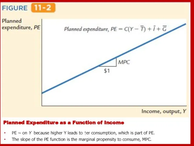
- 10. Planned Expenditure as a Function of Income PE ~ on Y because higher Y leads to
- 11. 11-1 The Goods Market and the IS Curve The Keynesian Cross The Interest Rate, Investment, and
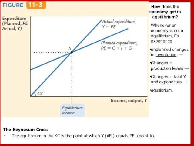
- 12. The Keynesian Cross The equilibrium in the KC is the point at which Y (AE )
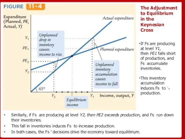
- 13. The Adjustment to Equilibrium in the Keynesian Cross Similarly, if Fs are producing at level Y2,
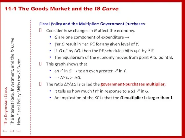
- 14. Fiscal Policy and the Multiplier: Government Purchases Consider how changes in G affect the economy. G
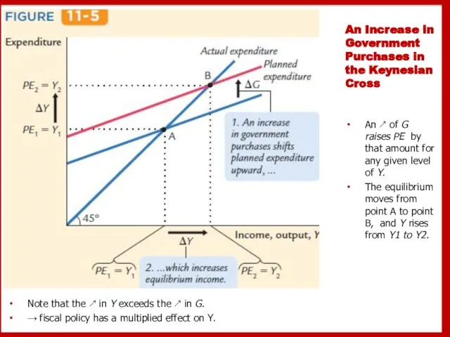
- 15. An Increase in Government Purchases in the Keynesian Cross Note that the ↗ in Y exceeds
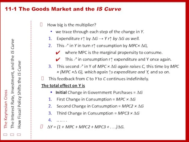
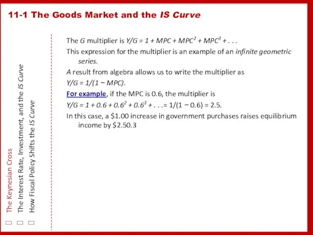
- 16. How big is the multiplier? we trace through each step of the change in Y. Expenditure
- 17. The Keynesian Cross The Interest Rate, Investment, and the IS Curve How Fiscal Policy Shifts the
- 18. Fiscal Policy and the Multiplier: Taxes A ↘in T of ∆T immediately r↑ disposable income Y
- 19. A Decrease in Taxes in the Keynesian Cross A ↘ in T of ∆T r↑ PE
- 20. John F. Kennedy became president of the United States in 1961. One of the council’s first
- 21. When President Barack Obama took office in January 2009, the economy was suffering from a significant
- 22. The KС explains the economy’s AD curve shows how the spending plans of H, F, the
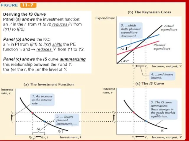
- 23. Deriving the IS Curve Panel (a) shows the investment function: an ↗ in the r from
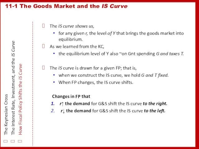
- 24. The IS curve shows us, for any given r, the level of Y that brings the
- 25. An Increase in Government Purchases Shifts the IS Curve Outward Panel (a) shows that an ↗
- 26. 11-2 The Money Market and the LM Curve The Theory of Liquidity Preference Income, Money Demand,
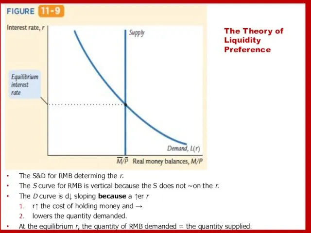
- 27. The Theory of Liquidity Preference The S&D for RMB determing the r. The S curve for
- 28. A Reduction in the Money Supply in the Theory of Liquidity Preference If the P is
- 29. Does a Monetary Tightening Raise or Lower Interest Rates?
- 30. 11-2 The Money Market and the LM Curve The Theory of Liquidity Preference Income, Money Demand,
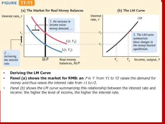
- 31. Deriving the LM Curve Panel (a) shows the market for RMB: an ↗ in Y from
- 32. The LM curve shows the combinations of the interest rate and the level of Y that
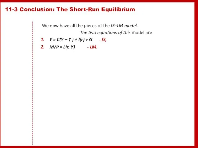
- 34. We now have all the pieces of the IS–LM model. The two equations of this model
- 35. The intersection of the IS and LM curves represents simultaneous equilibrium in the market for G&S
- 36. The Theory of Short-Run Fluctuations This schematic diagram shows how the different pieces of the theory
- 38. Скачать презентацию
11-1 The Goods Market and the IS Curve
11-2 The Money
11-1 The Goods Market and the IS Curve
11-2 The Money
Aggregate Demand I: Building the IS–LM Model
Classical theory (Ch.3-7) seemed incapable
Aggregate Demand I: Building the IS–LM Model
Classical theory (Ch.3-7) seemed incapable
Aggregate Demand I: Building the IS–LM Model
Our goal is
to identify
Aggregate Demand I: Building the IS–LM Model
Our goal is
to identify
Aggregate Demand I: Building the IS–LM Model
Shifts in Aggregate Demand
For a
Aggregate Demand I: Building the IS–LM Model
Shifts in Aggregate Demand
For a
The two parts of the IS–LM model
the IS curve
The two parts of the IS–LM model
the IS curve
The IS curve plots the relationship between the r & the
The IS curve plots the relationship between the r & the
11-1 The Goods Market and the IS Curve
The Keynesian Cross
11-1 The Goods Market and the IS Curve
The Keynesian Cross
11-1 The Goods Market and the IS Curve
The Keynesian Cross
11-1 The Goods Market and the IS Curve
The Keynesian Cross
Planned Expenditure as a Function of Income
PE ~ on Y because
Planned Expenditure as a Function of Income
PE ~ on Y because
11-1 The Goods Market and the IS Curve
The Keynesian Cross
11-1 The Goods Market and the IS Curve
The Keynesian Cross
The Keynesian Cross
The equilibrium in the KC is the point
The Keynesian Cross
The equilibrium in the KC is the point
The Adjustment to Equilibrium in the Keynesian Cross
Similarly, if Fs
The Adjustment to Equilibrium in the Keynesian Cross
Similarly, if Fs
Fiscal Policy and the Multiplier: Government Purchases
Consider how changes in
Fiscal Policy and the Multiplier: Government Purchases
Consider how changes in
An Increase in Government Purchases in the Keynesian Cross
Note that the
An Increase in Government Purchases in the Keynesian Cross
Note that the
How big is the multiplier?
we trace through each step of the
How big is the multiplier?
we trace through each step of the
The Keynesian Cross
The Interest Rate, Investment, and the IS Curve
The Keynesian Cross
The Interest Rate, Investment, and the IS Curve
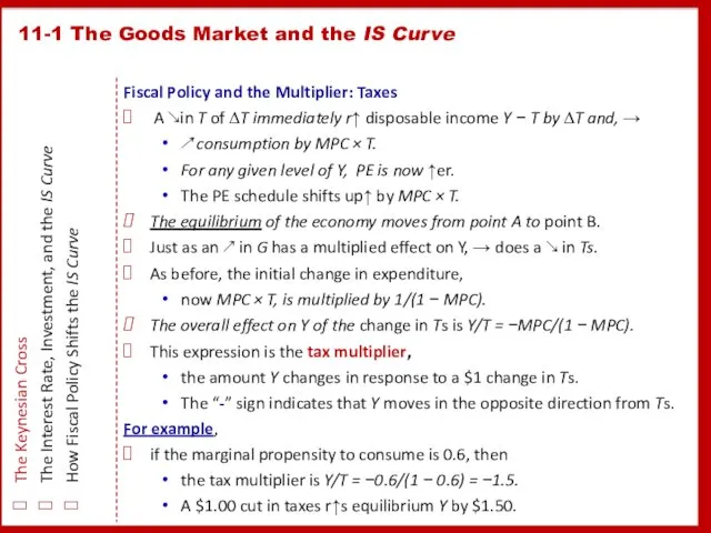
Fiscal Policy and the Multiplier: Taxes
A ↘in T of
Fiscal Policy and the Multiplier: Taxes
A ↘in T of
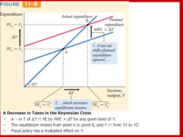
A Decrease in Taxes in the Keynesian Cross
A ↘ in
A Decrease in Taxes in the Keynesian Cross
A ↘ in
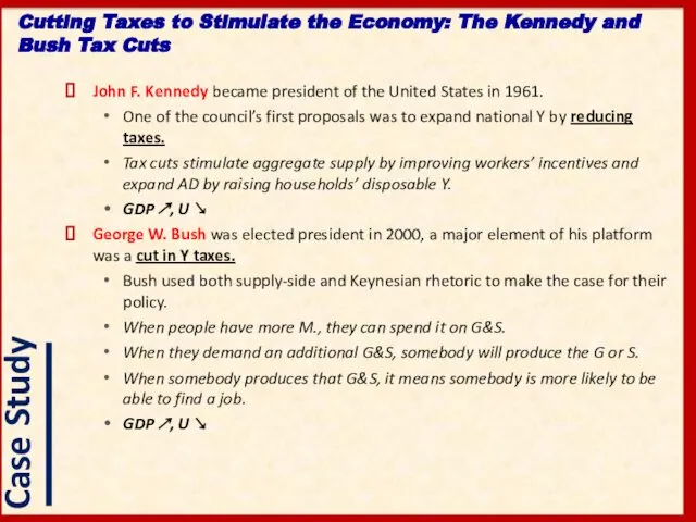
John F. Kennedy became president of the United States in 1961.
One
John F. Kennedy became president of the United States in 1961.
One
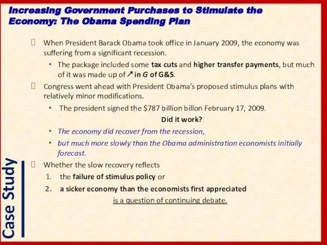
When President Barack Obama took office in January 2009, the economy
When President Barack Obama took office in January 2009, the economy
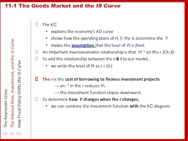
The KС
explains the economy’s AD curve
shows how the spending plans
The KС
explains the economy’s AD curve
shows how the spending plans
Deriving the IS Curve
Panel (a) shows the investment function:
an
Deriving the IS Curve
Panel (a) shows the investment function:
an
The IS curve shows us,
for any given r, the level
The IS curve shows us,
for any given r, the level
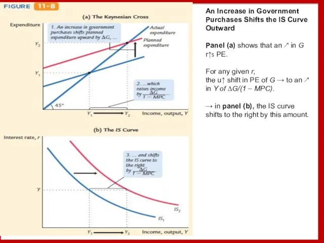
An Increase in Government Purchases Shifts the IS Curve Outward
Panel (a)
An Increase in Government Purchases Shifts the IS Curve Outward
Panel (a)
11-2 The Money Market and the LM Curve
The Theory of Liquidity
11-2 The Money Market and the LM Curve
The Theory of Liquidity
The Theory of Liquidity Preference
The S&D for RMB determing the r.
The
The Theory of Liquidity Preference
The S&D for RMB determing the r.
The
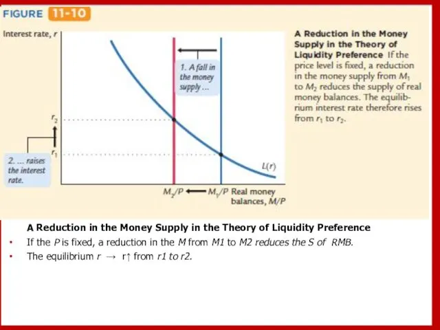
A Reduction in the Money Supply in the Theory of Liquidity
A Reduction in the Money Supply in the Theory of Liquidity
Does a Monetary Tightening Raise or Lower Interest Rates?
Does a Monetary Tightening Raise or Lower Interest Rates?
11-2 The Money Market and the LM Curve
The Theory of Liquidity
11-2 The Money Market and the LM Curve
The Theory of Liquidity
Deriving the LM Curve
Panel (a) shows the market for RMB:
Deriving the LM Curve
Panel (a) shows the market for RMB:
The LM curve shows the combinations of the interest rate and
The LM curve shows the combinations of the interest rate and

We now have all the pieces of the IS–LM model.
The
We now have all the pieces of the IS–LM model.
The
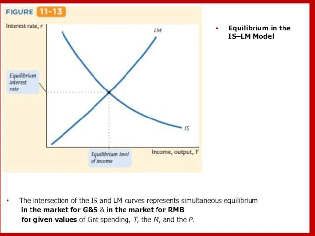
The intersection of the IS and LM curves represents simultaneous equilibrium
The intersection of the IS and LM curves represents simultaneous equilibrium
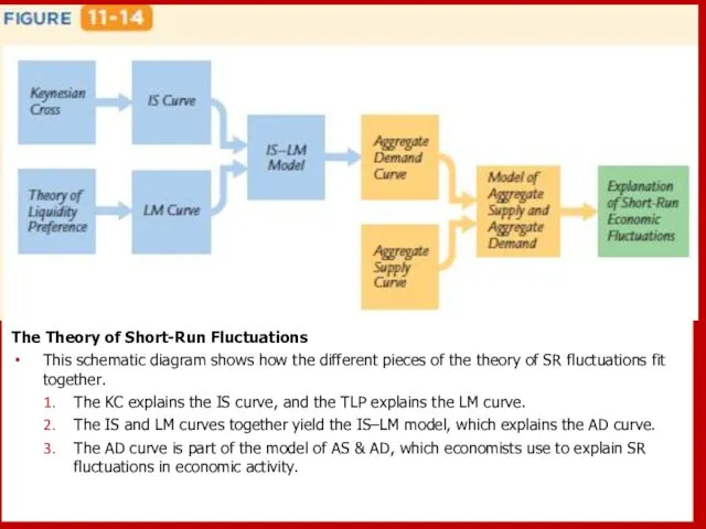
The Theory of Short-Run Fluctuations
This schematic diagram shows how the
The Theory of Short-Run Fluctuations
This schematic diagram shows how the
 Основные факторы современного развития туризма
 Інноваційно-технологічний ресурс глобального економічного розвитку
 Система комплексного экономического анализа
 Суды пайдалану Коммерциялық балық аулау
 Диверсификация. Стратегии диверсификации
 ОАО Агрокомбинат "Юбилейный"
 Управление проектами
 Экономика Центральной России
 Синергия. Синергетические эффекты
 Система оценки качества продукции в производстве
 Игра Что? Где? Когда? по экономике
 15 тақырып. Шет елдердегі баға құру және бағаларды реттеу тәжірибесі
 Экономика семьи
 Специфика и следствия российского монополизма
 Зарождение экономической науки
 Внешние эффекты и права собственности
 Принципы Ямайской валютной системы
 Налогово-бюджетная политика
 Рынок на практике, или как реально организована торговля
 Международная экономика и международные экономические отношения
 Кривая предложения. Закон предложения. Факторы предложения
 Организация продовольственной обороны РФ
 Эконометрика. Эконометрические модели. Простейшие модели временных рядов. Семинар 3
 Денсаулық сақтау экономикасы
 Движения антиглобалистов и альтерглобалистов как ответная реакция на процесс глобализации
 Игорь Ансофф
 Доклад об итогах социально-экономического развития Лотошинского муниципального района за 2017 год
 Государственное регулирование экономики