- Depressions and Slumps

Содержание
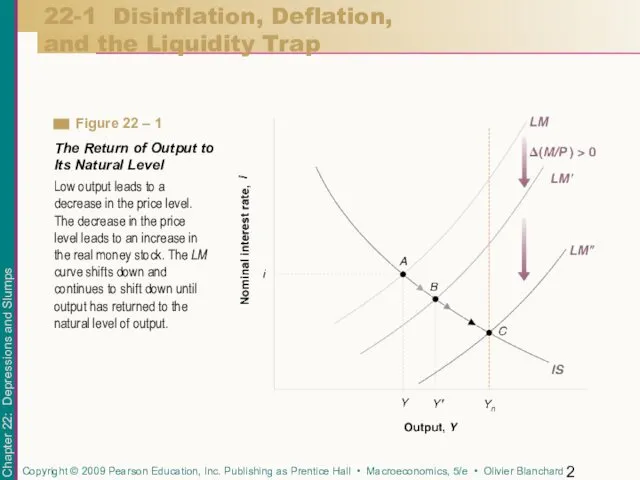
- 2. 22-1 Disinflation, Deflation, and the Liquidity Trap Low output leads to a decrease in the price
- 3. Recall from Chapter 7 and this graph that: Output is now below the natural level of
- 4. Chapters 8 and 9 presented a more realistic version of the model. Suppose output is below
- 5. The built-in mechanism that can lift economies out of recessions is this: Output below the natural
- 6. Recall from Chapter 14 that: What matters for spending decisions, and thus what enters the IS
- 7. 22-1 Disinflation, Deflation, and the Liquidity Trap The Nominal Interest Rate, the Real Interest Rate, and
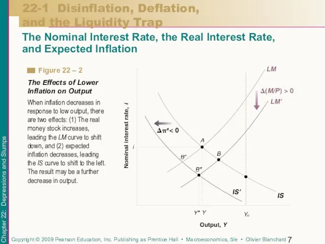
- 8. Because output is below the natural level of output, inflation falls. The decrease in inflation now
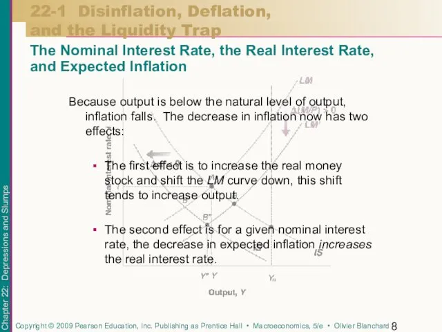
- 9. 22-1 Disinflation, Deflation, and the Liquidity Trap The Liquidity Trap When the nominal interest rate is
- 10. The demand for money is as shown in Figure 22-3. As the nominal interest rate decreases,
- 11. Now consider the effects of an increase in the money supply: Starting from the equilibrium of
- 12. The liquidity trap describes a situation in which expansionary monetary policy becomes powerless. The increase in
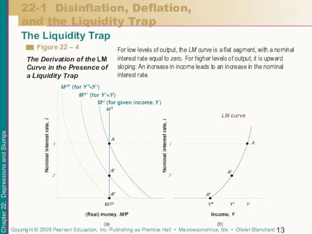
- 13. 22-1 Disinflation, Deflation, and the Liquidity Trap The Liquidity Trap For low levels of output, the
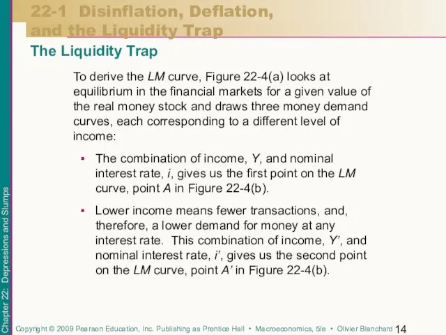
- 14. 22-1 Disinflation, Deflation, and the Liquidity Trap The Liquidity Trap To derive the LM curve, Figure
- 15. 22-1 Disinflation, Deflation, and the Liquidity Trap The Liquidity Trap The equilibrium is given by point
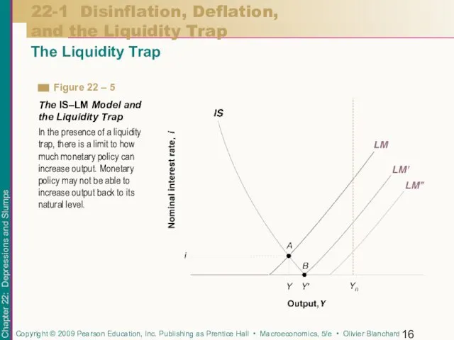
- 16. 22-1 Disinflation, Deflation, and the Liquidity Trap The Liquidity Trap In the presence of a liquidity
- 17. At a negative real interest rate of 10%, consumption and investment are likely to be very
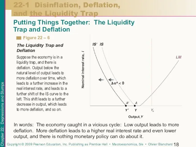
- 18. 22-1 Disinflation, Deflation, and the Liquidity Trap Putting Things Together: The Liquidity Trap and Deflation In
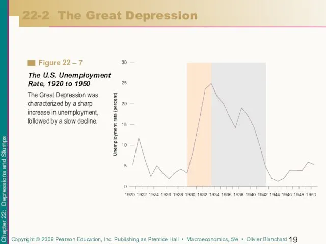
- 19. 22-2 The Great Depression The Great Depression was characterized by a sharp increase in unemployment, followed
- 20. 22-2 The Great Depression
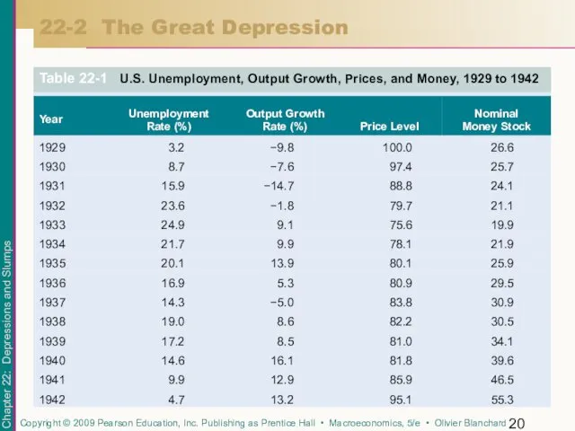
- 21. Focusing only on unemployment and output for the moment, two facts emerge from the table: How
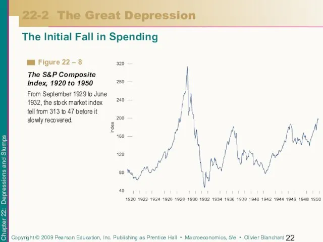
- 22. The Initial Fall in Spending 22-2 The Great Depression From September 1929 to June 1932, the
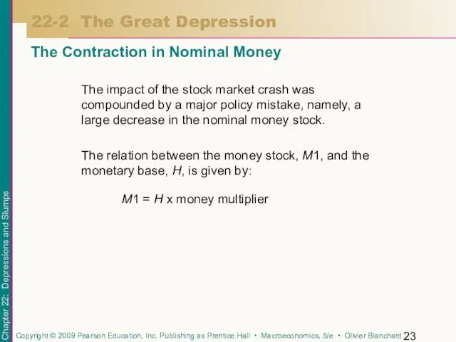
- 23. The Contraction in Nominal Money 22-2 The Great Depression The impact of the stock market crash
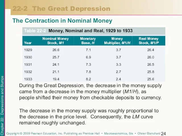
- 24. The Contraction in Nominal Money 22-2 The Great Depression During the Great Depression, the decrease in
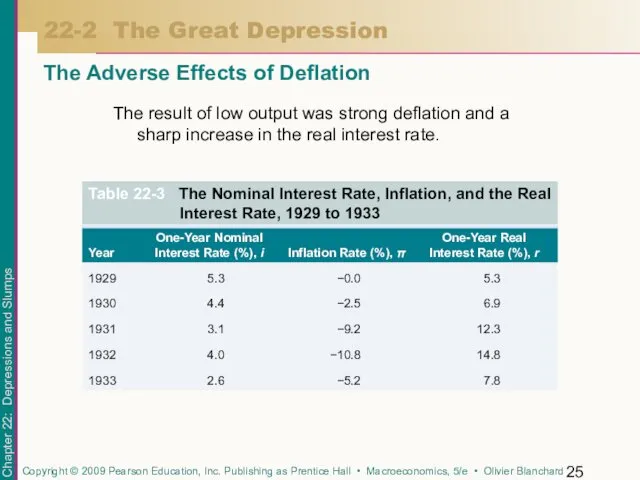
- 25. The result of low output was strong deflation and a sharp increase in the real interest
- 26. Monetary policy played an important role in the recovery. From 1933 to 1941, the nominal money
- 27. The puzzle is why deflation ended in 1933. One proximate cause may be the set of
- 28. The robust growth that Japan had experienced since the end of World War II came to
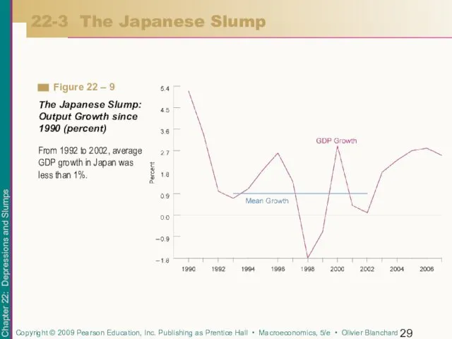
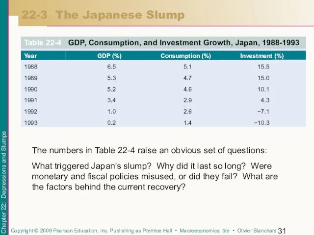
- 29. 22-3 The Japanese Slump From 1992 to 2002, average GDP growth in Japan was less than
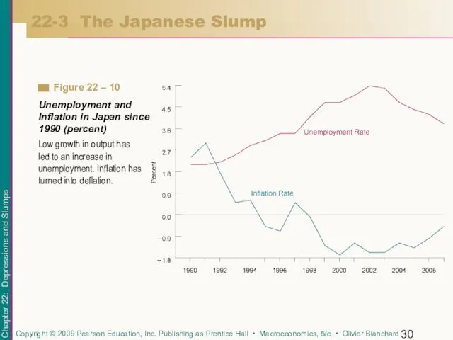
- 30. 22-3 The Japanese Slump Low growth in output has led to an increase in unemployment. Inflation
- 31. 22-3 The Japanese Slump The numbers in Table 22-4 raise an obvious set of questions: What
- 32. There are two reasons for the increase in a stock price: A change in the fundamental
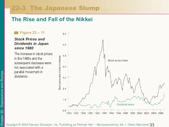
- 33. 22-3 The Japanese Slump The Rise and Fall of the Nikkei The increase in stock prices
- 34. The fact that dividends remained flat while stock prices increased strongly suggests that a large bubble
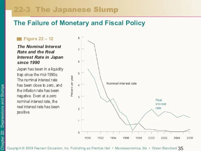
- 35. 22-3 The Japanese Slump The Failure of Monetary and Fiscal Policy Japan has been in a
- 36. Monetary policy was used, but it was used too late, and when it was used, if
- 37. Fiscal policy was used as well. Taxes decreased at the start of the slump, and there
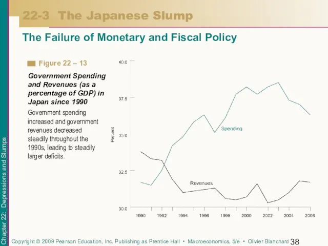
- 38. 22-3 The Japanese Slump The Failure of Monetary and Fiscal Policy Government spending increased and government
- 39. Output growth has been higher since 2003, and most economists cautiously predict that the recovery will
- 40. It is suggested that even if the nominal interest rate is already equal to zero and
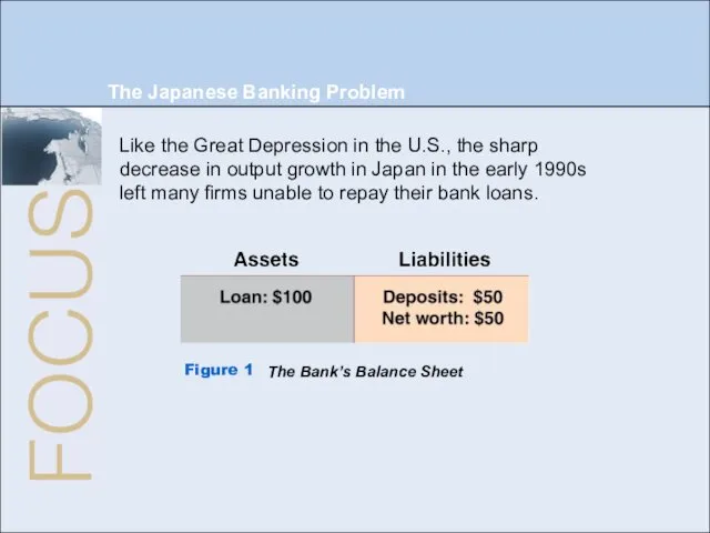
- 41. The Japanese Banking Problem Like the Great Depression in the U.S., the sharp decrease in output
- 43. Скачать презентацию
22-1 Disinflation, Deflation,
and the Liquidity Trap
Low output leads to a decrease
22-1 Disinflation, Deflation,
and the Liquidity Trap
Low output leads to a decrease
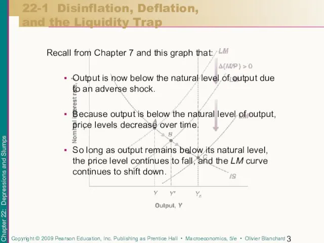
Recall from Chapter 7 and this graph that:
Output is now below
Recall from Chapter 7 and this graph that:
Output is now below
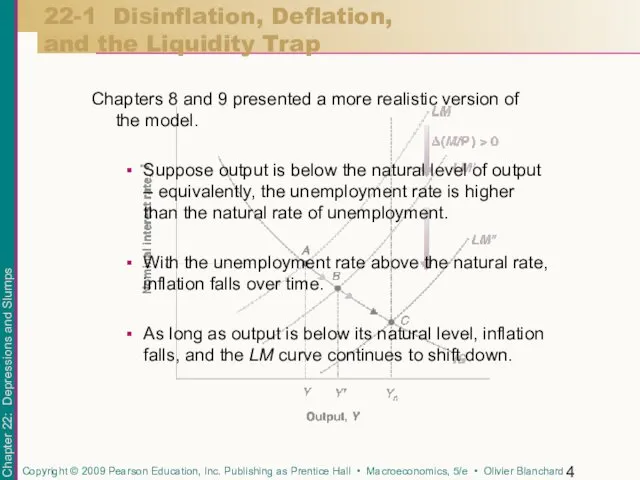
Chapters 8 and 9 presented a more realistic version of the
Chapters 8 and 9 presented a more realistic version of the
The built-in mechanism that can lift economies out of recessions is
The built-in mechanism that can lift economies out of recessions is
Recall from Chapter 14 that:
What matters for spending decisions, and thus
Recall from Chapter 14 that:
What matters for spending decisions, and thus
22-1 Disinflation, Deflation,
and the Liquidity Trap
The Nominal Interest Rate, the Real
22-1 Disinflation, Deflation,
and the Liquidity Trap
The Nominal Interest Rate, the Real
Because output is below the natural level of output, inflation falls.
Because output is below the natural level of output, inflation falls.
22-1 Disinflation, Deflation,
and the Liquidity Trap
The Liquidity Trap
When the nominal interest
22-1 Disinflation, Deflation,
and the Liquidity Trap
The Liquidity Trap
When the nominal interest

The demand for money is as shown in Figure 22-3.
As the
The demand for money is as shown in Figure 22-3.
As the
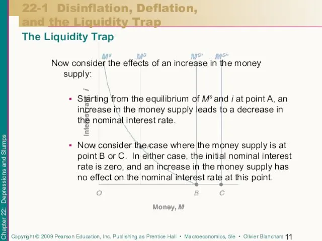
Now consider the effects of an increase in the money supply:
Starting
Now consider the effects of an increase in the money supply:
Starting
The liquidity trap describes a situation in which expansionary monetary policy
The liquidity trap describes a situation in which expansionary monetary policy
22-1 Disinflation, Deflation,
and the Liquidity Trap
The Liquidity Trap
For low levels of
22-1 Disinflation, Deflation,
and the Liquidity Trap
The Liquidity Trap
For low levels of
22-1 Disinflation, Deflation,
and the Liquidity Trap
The Liquidity Trap
To derive the LM
22-1 Disinflation, Deflation,
and the Liquidity Trap
The Liquidity Trap
To derive the LM
22-1 Disinflation, Deflation,
and the Liquidity Trap
The Liquidity Trap
The equilibrium is given
22-1 Disinflation, Deflation,
and the Liquidity Trap
The Liquidity Trap
The equilibrium is given
22-1 Disinflation, Deflation,
and the Liquidity Trap
The Liquidity Trap
In the presence of
22-1 Disinflation, Deflation,
and the Liquidity Trap
The Liquidity Trap
In the presence of
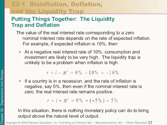
At a negative real interest rate of 10%, consumption and investment
At a negative real interest rate of 10%, consumption and investment
22-1 Disinflation, Deflation,
and the Liquidity Trap
Putting Things Together: The Liquidity
Trap
22-1 Disinflation, Deflation,
and the Liquidity Trap
Putting Things Together: The Liquidity Trap
22-2 The Great Depression
The Great Depression was characterized by a sharp
22-2 The Great Depression
The Great Depression was characterized by a sharp
22-2 The Great Depression
22-2 The Great Depression
Focusing only on unemployment and output for the moment, two facts
Focusing only on unemployment and output for the moment, two facts
The Initial Fall in Spending
22-2 The Great Depression
From September 1929 to
The Initial Fall in Spending
22-2 The Great Depression
From September 1929 to
The Contraction in Nominal Money
22-2 The Great Depression
The impact of the
The Contraction in Nominal Money
22-2 The Great Depression
The impact of the
The Contraction in Nominal Money
22-2 The Great Depression
During the Great Depression,
The Contraction in Nominal Money
22-2 The Great Depression
During the Great Depression,
The result of low output was strong deflation and a sharp
The result of low output was strong deflation and a sharp
Monetary policy played an important role in the recovery. From 1933
Monetary policy played an important role in the recovery. From 1933
The puzzle is why deflation ended in 1933.
One proximate cause may
The puzzle is why deflation ended in 1933.
One proximate cause may
The robust growth that Japan had experienced since the end of
The robust growth that Japan had experienced since the end of
22-3 The Japanese Slump
From 1992 to 2002, average GDP growth in
22-3 The Japanese Slump
From 1992 to 2002, average GDP growth in
22-3 The Japanese Slump
Low growth in output has led to an
22-3 The Japanese Slump
Low growth in output has led to an
22-3 The Japanese Slump
The numbers in Table 22-4 raise an obvious
22-3 The Japanese Slump
The numbers in Table 22-4 raise an obvious
There are two reasons for the increase in a stock price:
A
There are two reasons for the increase in a stock price:
A
22-3 The Japanese Slump
The Rise and Fall of the Nikkei
The increase
22-3 The Japanese Slump
The Rise and Fall of the Nikkei
The increase
The fact that dividends remained flat while stock prices increased strongly
The fact that dividends remained flat while stock prices increased strongly
22-3 The Japanese Slump
The Failure of Monetary and Fiscal Policy
Japan has
22-3 The Japanese Slump
The Failure of Monetary and Fiscal Policy
Japan has
Monetary policy was used, but it was used too late, and
Monetary policy was used, but it was used too late, and
Fiscal policy was used as well. Taxes decreased at the start
Fiscal policy was used as well. Taxes decreased at the start
22-3 The Japanese Slump
The Failure of Monetary and Fiscal Policy
Government spending
22-3 The Japanese Slump
The Failure of Monetary and Fiscal Policy
Government spending
Output growth has been higher since 2003, and most economists cautiously
Output growth has been higher since 2003, and most economists cautiously
It is suggested that even if the nominal interest rate is
It is suggested that even if the nominal interest rate is
The Japanese Banking Problem
Like the Great Depression in the U.S., the
The Japanese Banking Problem
Like the Great Depression in the U.S., the
 Понятие предприятия
 Статистические методы изучения взаимосвязи социально-экономических явлений. (Лекция 4)
 Світове господарство та етапи його формування. 10 клас
 Экономическая теория. Введение в макроэкономику. Система национальных счетов. (Модуль 2.1)
 Кризис как фактор жизнедеятельности социально-экономических систем
 Структурная перестройка в экономике РФ
 Внешнеторговые показатели в международной торговле
 Асимметричность информации и отношения «принципал-агент»
 Модель межотраслевого баланса
 Особенности, динамика, перспективы внешнеэкономических связей Ростовской области
 Экспорт российской продукции АПК
 Экономический морской бой
 Проблема занятости молодежи
 Проект экономика родного края (село Бабяково)
 Правила обращения за региональной социальной доплатой к пенсии, порядок ее установления, выплаты и пересмотра ее размера
 Теория отраслевых рынков
 Инвестиции и инвестиционная деятельность
 Программа по выходу из кризиса города Возрождения
 Основные Средства
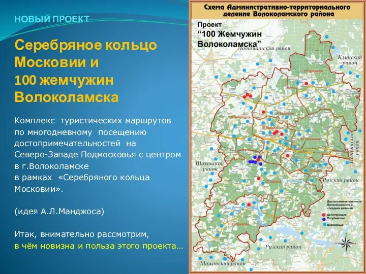 Комплекс туристических маршрутов по многодневному посещению достопримечательностей в рамках «Серебряного кольца Московии»
 Самые популярные профессии Ростова-на-Дону
 Учет оборотных активов. (Тема 5)
 Теория производства и предельной производительности факторов (первая часть)
 Экономическая теория
 Экономические системы А. Смита и Д. Рикардо
 Практичне застосування GJR model в Азії
 Российский морской регистр судоходства
 Социальная политика государства и управление социальным развитием организации. Россия и Сингапур