- The Elasticity of supply and demand

Содержание
- 2. ELASTICITY: A MEASURE OF RESPONSE Imagine that you are the manager of the public transportation system
- 3. THE PRICE ELASTICITY OF DEMAND
- 4. NB: With a downward-sloping demand curve, price and quantity demanded move in opposite directions, so the
- 5. COMPUTING THE PRICE ELASTICITY OF DEMAND Finding the price elasticity of demand requires that we first
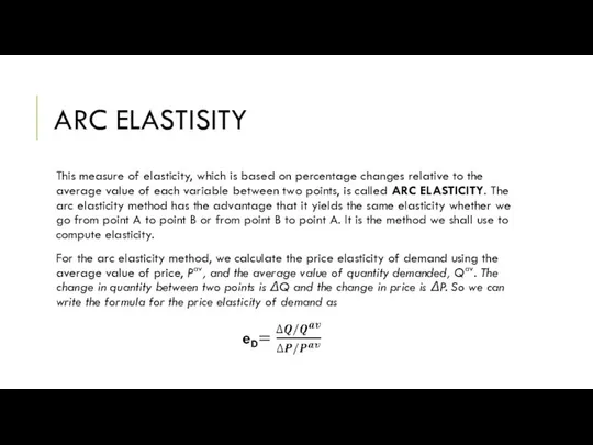
- 6. ARC ELASTISITY This measure of elasticity, which is based on percentage changes relative to the average
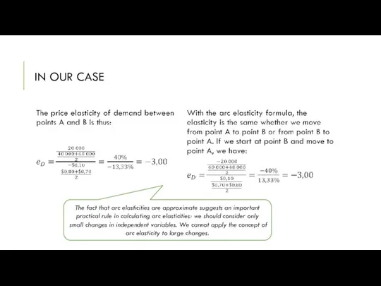
- 7. IN OUR CASE The fact that arc elasticities are approximate suggests an important practical rule in
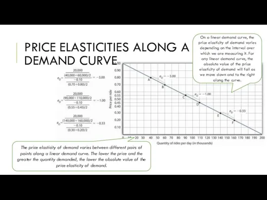
- 8. PRICE ELASTICITIES ALONG A LINEAR DEMAND CURVE The price elasticity of demand varies between different pairs
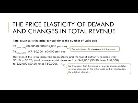
- 9. THE PRICE ELASTICITY OF DEMAND AND CHANGES IN TOTAL REVENUE Total revenue is the price per
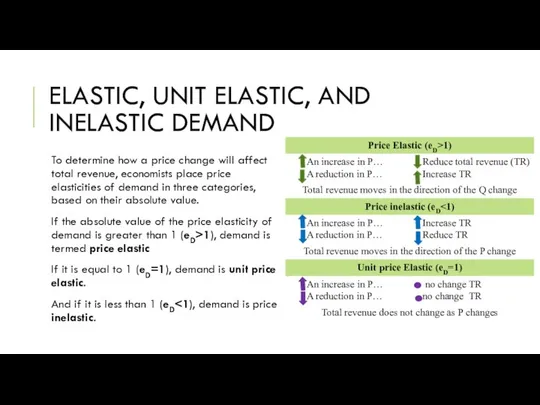
- 10. ELASTIC, UNIT ELASTIC, AND INELASTIC DEMAND To determine how a price change will affect total revenue,
- 11. For any linear demand curve, demand will be price elastic in the upper half of the
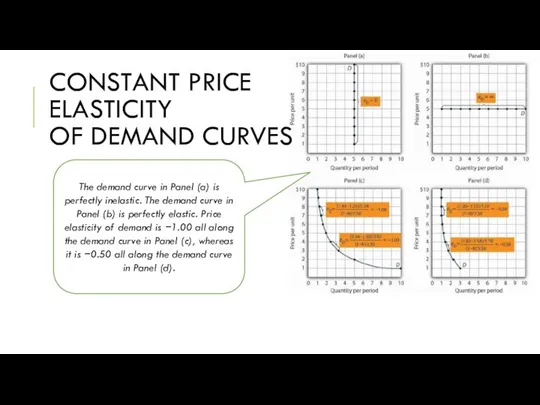
- 12. CONSTANT PRICE ELASTICITY OF DEMAND CURVES The demand curve in Panel (a) is perfectly inelastic. The
- 13. DETERMINANTS OF THE PRICE ELASTICITY OF DEMAND Availability of Substitutes (The availability of close substitutes tends
- 14. SUMMARY The price elasticity of demand measures the responsiveness of quantity demanded to changes in price;
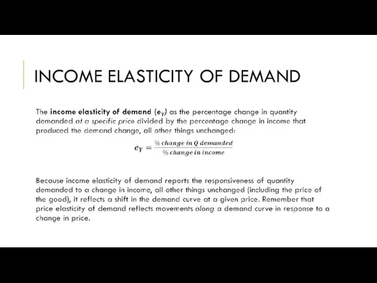
- 15. INCOME ELASTICITY OF DEMAND
- 16. A positive income elasticity of demand means that income and demand move in the same direction—an
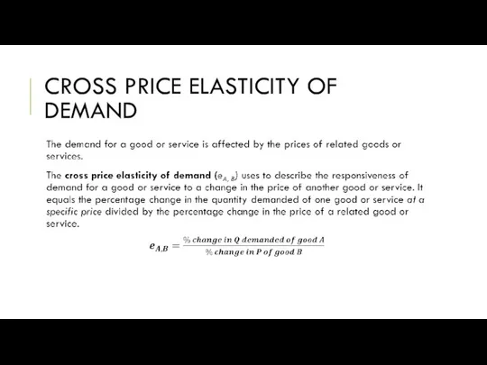
- 17. CROSS PRICE ELASTICITY OF DEMAND
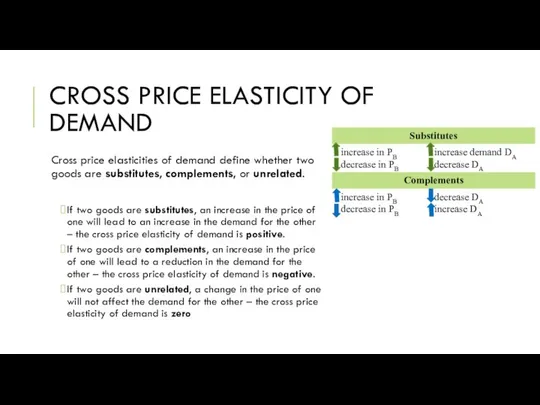
- 18. CROSS PRICE ELASTICITY OF DEMAND Cross price elasticities of demand define whether two goods are substitutes,
- 19. SUMMARY The income elasticity of demand reflects the responsiveness of demand to changes in income. It
- 20. PRICE ELASTICITY OF SUPPLY Price elasticity of supply as the ratio of the percentage change in
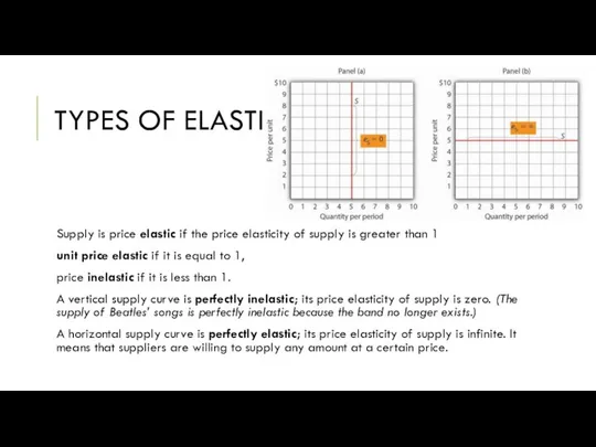
- 21. TYPES OF ELASTICITY Supply is price elastic if the price elasticity of supply is greater than
- 22. APPLICATION S2 – a supply curve in which quantity supplied is more responsive to price changes
- 24. Скачать презентацию
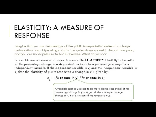
ELASTICITY: A MEASURE OF RESPONSE
Imagine that you are the manager of
ELASTICITY: A MEASURE OF RESPONSE
Imagine that you are the manager of
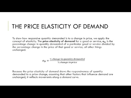
THE PRICE ELASTICITY OF DEMAND
THE PRICE ELASTICITY OF DEMAND
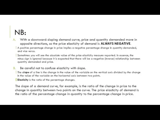
NB:
With a downward-sloping demand curve, price and quantity demanded move in
NB:
With a downward-sloping demand curve, price and quantity demanded move in
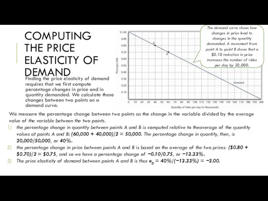
COMPUTING THE PRICE ELASTICITY OF DEMAND
Finding the price elasticity of
COMPUTING THE PRICE ELASTICITY OF DEMAND
Finding the price elasticity of
ARC ELASTISITY
This measure of elasticity, which is based on percentage changes
ARC ELASTISITY
This measure of elasticity, which is based on percentage changes
IN OUR CASE
The fact that arc elasticities are approximate suggests an
IN OUR CASE
The fact that arc elasticities are approximate suggests an
PRICE ELASTICITIES ALONG A LINEAR
DEMAND CURVE
The price elasticity of demand
PRICE ELASTICITIES ALONG A LINEAR
DEMAND CURVE
The price elasticity of demand
THE PRICE ELASTICITY OF DEMAND AND CHANGES IN TOTAL REVENUE
Total revenue
THE PRICE ELASTICITY OF DEMAND AND CHANGES IN TOTAL REVENUE
Total revenue
ELASTIC, UNIT ELASTIC, AND INELASTIC DEMAND
To determine how a price change
ELASTIC, UNIT ELASTIC, AND INELASTIC DEMAND
To determine how a price change
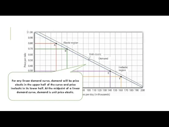
For any linear demand curve, demand will be price elastic in
For any linear demand curve, demand will be price elastic in
CONSTANT PRICE ELASTICITY
OF DEMAND CURVES
The demand curve in Panel (a)
CONSTANT PRICE ELASTICITY
OF DEMAND CURVES
The demand curve in Panel (a)

DETERMINANTS OF THE PRICE ELASTICITY OF DEMAND
Availability of Substitutes (The availability
DETERMINANTS OF THE PRICE ELASTICITY OF DEMAND
Availability of Substitutes (The availability

SUMMARY
The price elasticity of demand measures the responsiveness of quantity demanded
SUMMARY
The price elasticity of demand measures the responsiveness of quantity demanded
INCOME ELASTICITY OF DEMAND
INCOME ELASTICITY OF DEMAND
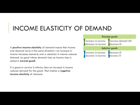
A positive income elasticity of demand means that income and demand
A positive income elasticity of demand means that income and demand
CROSS PRICE ELASTICITY OF DEMAND
CROSS PRICE ELASTICITY OF DEMAND
CROSS PRICE ELASTICITY OF DEMAND
Cross price elasticities of demand define whether
CROSS PRICE ELASTICITY OF DEMAND
Cross price elasticities of demand define whether

SUMMARY
The income elasticity of demand reflects the responsiveness of demand to
SUMMARY
The income elasticity of demand reflects the responsiveness of demand to

PRICE ELASTICITY OF SUPPLY
Price elasticity of supply as the ratio
PRICE ELASTICITY OF SUPPLY
Price elasticity of supply as the ratio
TYPES OF ELASTICITY
Supply is price elastic if the price elasticity of
TYPES OF ELASTICITY
Supply is price elastic if the price elasticity of
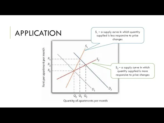
APPLICATION
S2 – a supply curve in which quantity supplied is more
APPLICATION
S2 – a supply curve in which quantity supplied is more
 Ішкішаруашылық жерге орналастыру
 Уровневый анализ объекта, предмета и метода современной экономической теории
 Кризис кейнсианства
 Уральский экономический район
 Экономическая теория. (Лекция 1)
 Теория провалов рынка и роль государства в рыночной экономике
 Либерализм, или классическая школа в политической экономике
 Анализ и совершенствование мониторинга рисков
 ВШЭУ Кафедра Финансы, денежное обращение и кредит. Направление подготовки: Экономика
 Планирования производства на сельскохозяйственных предприятиях. (Тема 3)
 Реформы С.Ю. Витте в сфере прямого и косвенного налогообложения
 Классификация инноваций
 Рыночная система и особенности ее функционирования. Виды рынков
 Глобализация и её последствия
 Государственный сектор. Макроэкономика Тема 5
 Особенности рынка фармацевтической продукции
 Финансы организаций. Оборотные средства. (Тема 3.3)
 Экономические индексы в статистике
 О подготовке к проведению статистического наблюдения за деятельностью субъектов малого и среднего предпринимательства
 Микроэкономика и макроэкономика
 Организация труда на предприятии
 Виды экономического анализа. Этапы его проведения
 Соотношения между темпами роста номинальных и реальных величин в дискретном и непрерывном времени
 Особенности накопления первоначального капитала Франции
 Экономическая безопасность предприятия. (Лекция 16)
 Презентация Должностной статус руководителя
 Дүние жүзілік шаруашылық
 Системы и системный подход