- Constant Jerk Trajectory Generator

Содержание
- 2. In particular, you will Determine why S-curves are necessary Review the ideal S-curve. Consider constant acceleration
- 3. Why S-curves? Reviewing the trapezoidal trajectory profile in speed v, we examine points 1, 2, 3,
- 4. Ideal S-curve t t = T vo vs v 1 as ar 1 Concave Convex t
- 5. Ideal S-curve equations The form assumed for the S-curve velocity profile is v(t) = co +
- 6. Concave period The concave conditions are v(0) = vo a(0) = 0 a(T/2) = as j(0)
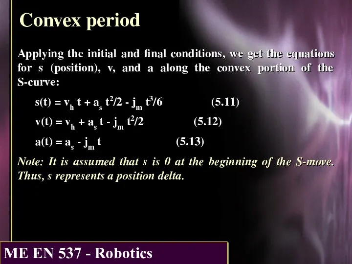
- 7. Concave period Applying the initial and final conditions, we get the equations for s (position), v,
- 8. Ideal S-curve observations If we let Δv = vs - vo and define ar = Δv/T
- 9. Convex period This period applies for T/2 ≤ t ≤ T. Letting time be zero measured
- 10. Convex period Applying the initial and final conditions, we get the equations for s (position), v,
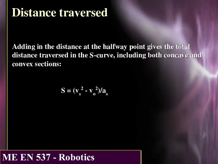
- 11. Distance traversed Adding in the distance at the halfway point gives the total distance traversed in
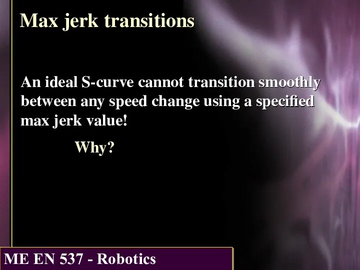
- 12. Max jerk transitions An ideal S-curve cannot transition smoothly between any speed change using a specified
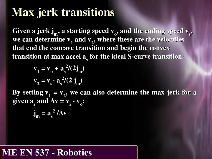
- 13. Max jerk transitions Given a jerk jm, a starting speed vo, and the ending speed vs,
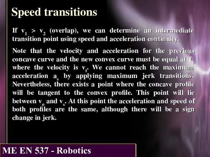
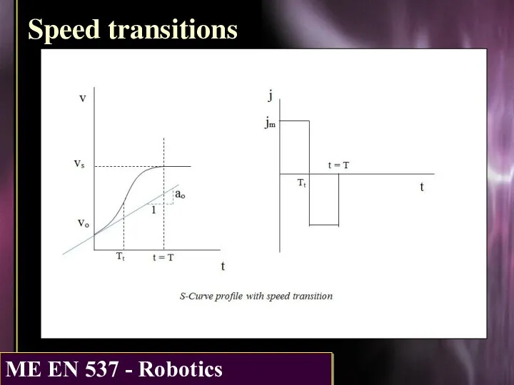
- 14. Speed transitions If v1 > v2 (overlap), we can determine an intermediate transition point using speed
- 15. Speed transitions
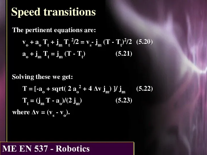
- 16. Speed transitions The pertinent equations are: vo + ao Tt + jm Tt 2/2 = vs-
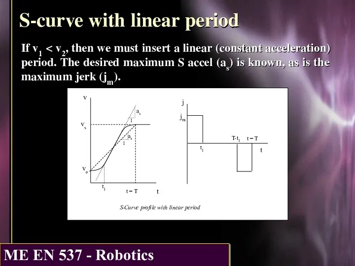
- 17. S-curve with linear period If v1
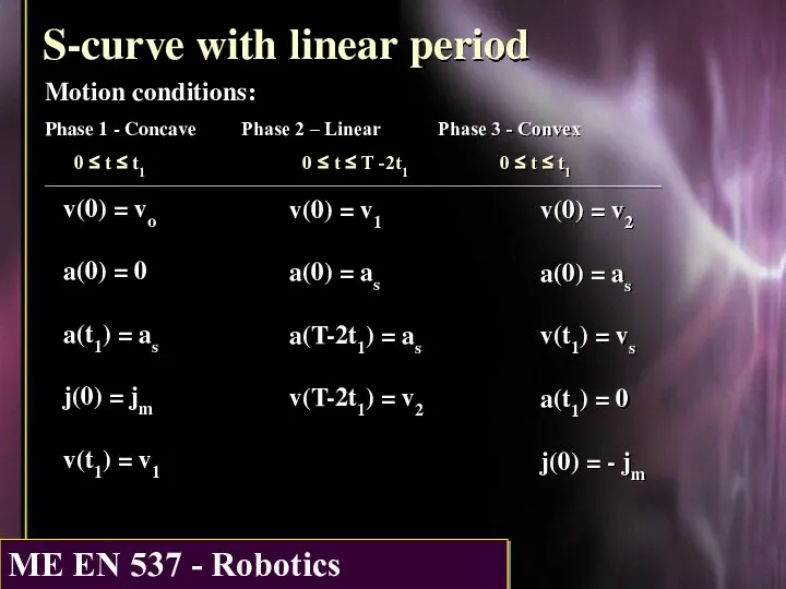
- 18. S-curve with linear period Motion conditions: Phase 1 - Concave Phase 2 – Linear Phase 3
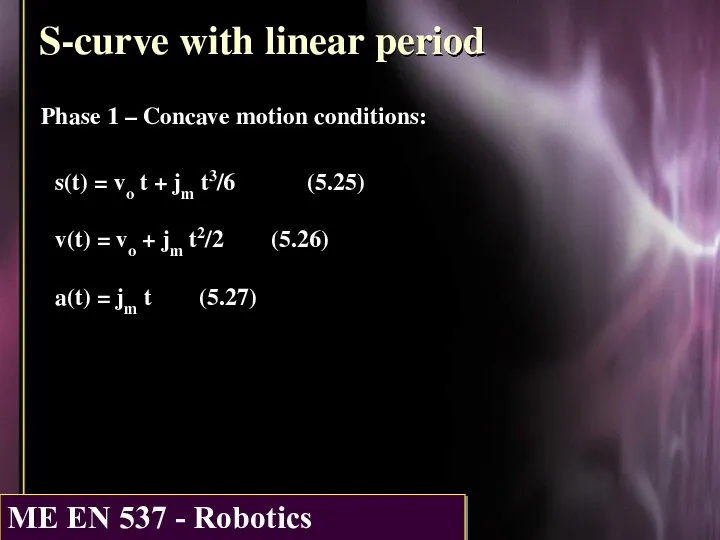
- 19. S-curve with linear period Phase 1 – Concave motion conditions: s(t) = vo t + jm
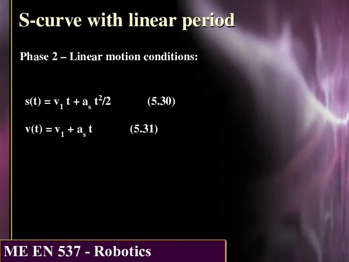
- 20. S-curve with linear period Phase 2 – Linear motion conditions: s(t) = v1 t + as
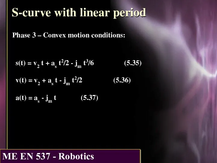
- 21. S-curve with linear period Phase 3 – Convex motion conditions: s(t) = v2 t + as
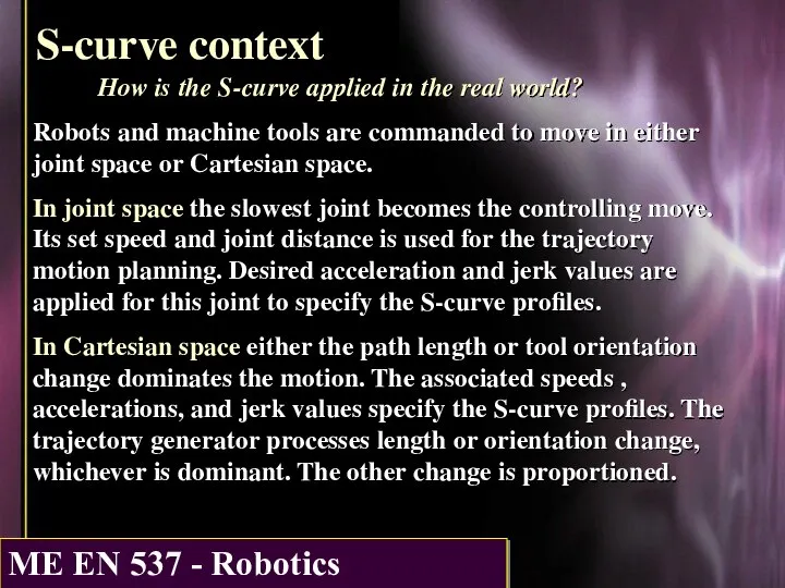
- 22. S-curve context How is the S-curve applied in the real world? Robots and machine tools are
- 24. Скачать презентацию
In particular, you will
Determine why S-curves are necessary
Review the ideal
In particular, you will
Determine why S-curves are necessary
Review the ideal
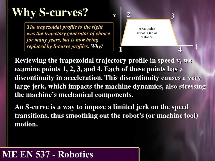
Why S-curves?
Reviewing the trapezoidal trajectory profile in speed v, we
Why S-curves?
Reviewing the trapezoidal trajectory profile in speed v, we
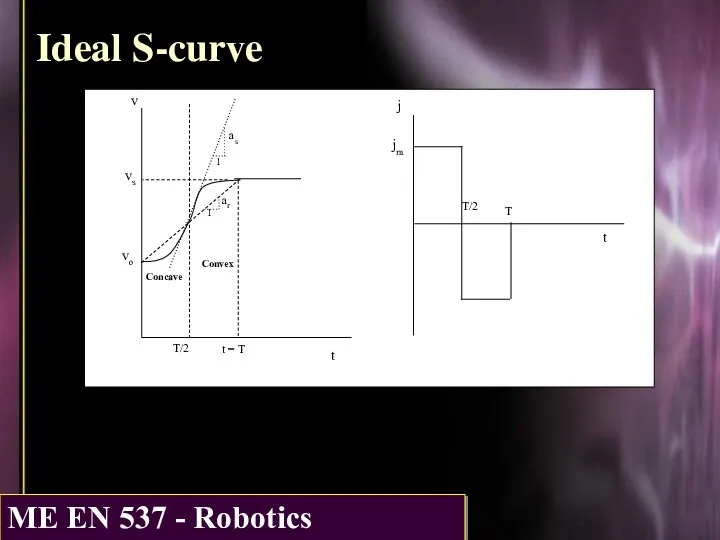
Ideal S-curve
t
t = T
vo
vs
v
1
as
ar
1
Concave
Convex
t
j
T/2
T/2
jm
T
Ideal S-curve
t
t = T
vo
vs
v
1
as
ar
1
Concave
Convex
t
j
T/2
T/2
jm
T
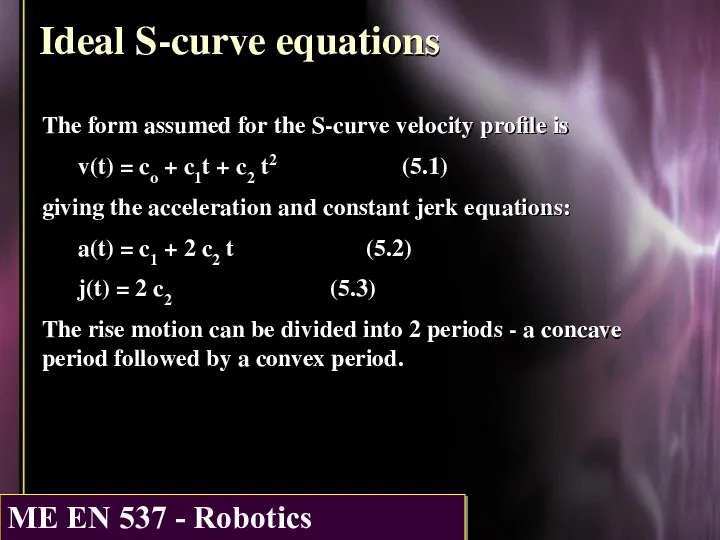
Ideal S-curve equations
The form assumed for the S-curve velocity profile
Ideal S-curve equations
The form assumed for the S-curve velocity profile
Concave period
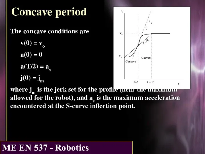
The concave conditions are
v(0) = vo
a(0) = 0
a(T/2) = as
j(0)
Concave period
The concave conditions are
v(0) = vo
a(0) = 0
a(T/2) = as
j(0)
Concave period
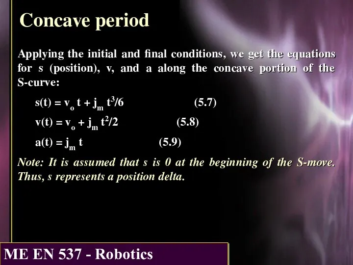
Applying the initial and final conditions, we get the equations
Concave period
Applying the initial and final conditions, we get the equations
Ideal S-curve observations
If we let Δv = vs - vo
Ideal S-curve observations
If we let Δv = vs - vo
Convex period
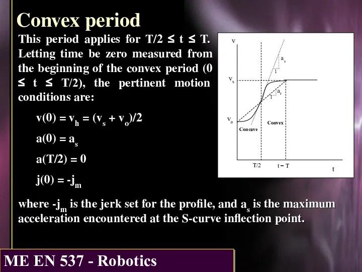
This period applies for T/2 ≤ t ≤ T. Letting
Convex period
This period applies for T/2 ≤ t ≤ T. Letting
Convex period
Applying the initial and final conditions, we get the equations
Convex period
Applying the initial and final conditions, we get the equations
Distance traversed
Adding in the distance at the halfway point gives
Distance traversed
Adding in the distance at the halfway point gives
Max jerk transitions
An ideal S-curve cannot transition smoothly between any
Max jerk transitions
An ideal S-curve cannot transition smoothly between any
Max jerk transitions
Given a jerk jm, a starting speed vo,
Max jerk transitions
Given a jerk jm, a starting speed vo,
Speed transitions
If v1 > v2 (overlap), we can determine an
Speed transitions
If v1 > v2 (overlap), we can determine an
Speed transitions
Speed transitions
Speed transitions
The pertinent equations are:
vo + ao Tt + jm
Speed transitions
The pertinent equations are:
vo + ao Tt + jm
S-curve with linear period
If v1 < v2, then we must insert
S-curve with linear period
If v1 < v2, then we must insert
S-curve with linear period
Motion conditions:
Phase 1 - Concave Phase 2 –
S-curve with linear period
Motion conditions:
Phase 1 - Concave Phase 2 –
S-curve with linear period
Phase 1 – Concave motion conditions:
s(t) = vo
S-curve with linear period
Phase 1 – Concave motion conditions:
s(t) = vo
S-curve with linear period
Phase 2 – Linear motion conditions:
s(t) = v1
S-curve with linear period
Phase 2 – Linear motion conditions:
s(t) = v1
S-curve with linear period
Phase 3 – Convex motion conditions:
s(t) = v2
S-curve with linear period
Phase 3 – Convex motion conditions:
s(t) = v2
S-curve context
How is the S-curve applied in the real world?
Robots
S-curve context
How is the S-curve applied in the real world?
Robots
 Реактивное движение
 Принцип действия радиотелефонной связи. Радиовещание и телевидение
  Презентация на тему: Тайна черной дыры!
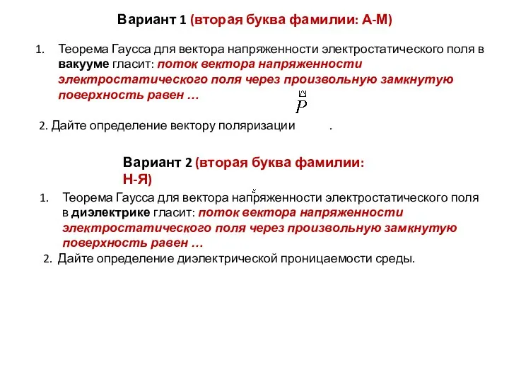 Варианты самостоятельной работы
 Динамика материальной точки. Лекция 3
 Презентация по физике "«Механическое движение тела»" - скачать
 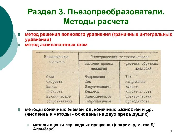 Пьезопреобразователи. Методы расчета. (Раздел 3)
 История развития материаловедения
 Ток күші. Амперметр. Электр кернеуі. Вольтметр
 Дифракция электромагнитной волны
 Даими магнитларның магнит кыры. дайм Жирнең магнит кыры
 Механизмы переноса тепла: теплопроводность, конвекция, излучение
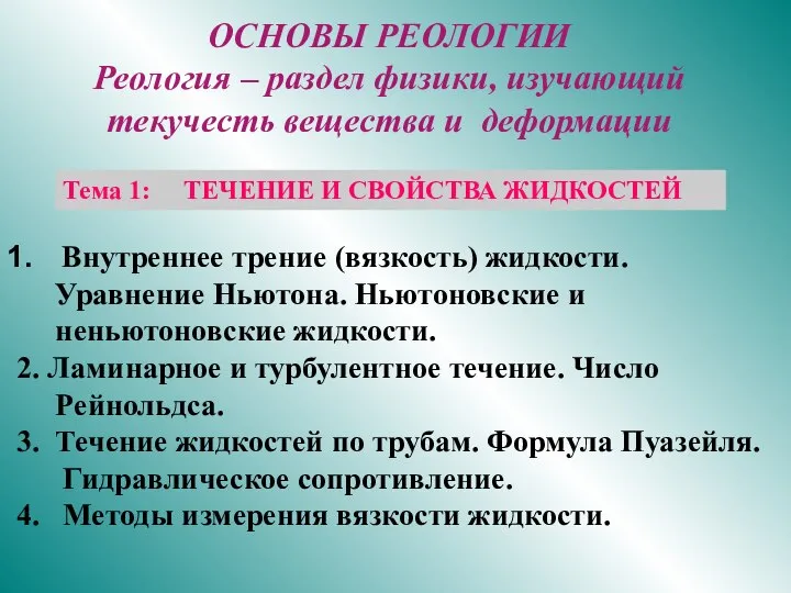 Реология. Течение и свойства жидкостей
 Основы специальной теории относительности
 Прозрачный люминесцентный солнечный концентратор
 Закон Кулона
 Использование энергии
 Одномерные изоэнтропные движения газа
 Объяснение электрических явлений
 Рівномірний рух по колу
 Фотоэффект. Теория фотоэффекта
 Введение в теорию конечных элементов
 Звуковые волны
 Вечный двигатель на капиллярном притяжение
 Методы изучения кинетики электродных процессов
 Техническое облуживание АКПП с гидравлическим приводом
 Проверка домашнего задания тест
 Плотность . Решение задач. Урок физики в 7 классе. Учитель Кононова Е.Ю.