- Point defects and diffusion

Содержание
- 2. Crystalline solids have a very regular atomic structure: that is, the local positions of atoms with
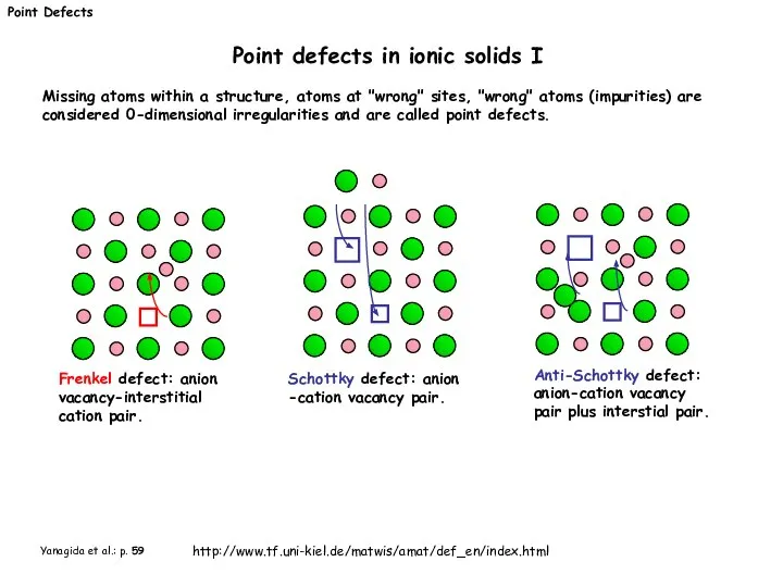
- 3. Point Defects Point defects in ionic solids I Frenkel defect: anion vacancy-interstitial cation pair. Schottky defect:
- 4. F-center: anion vacancy with excess electron replacing the missing anion e- M-center: two anion vacancies with
- 5. M corresonds to the species. These include: atoms - e.g. Si, Ni, O, Cl, vacancies -
- 6. Point Defects Kröger-Vink notation II = an aluminium ion sitting on an aluminium lattice site, with
- 7. Reaction involving defects must be: Example: Point Defects Defect chemical reaction Formation of a Schottky defect
- 8. Gperf: free energy of the perfect crystal hdef: enthalpy of formation of one defect sdvib: vibrational
- 9. Yanagida et al.: p. 60-61 Number of ways to arrange nv vacancies within a crystal with
- 10. Entropy Configurational Entropy Entropy originating from the many possibilities of arranging many vacancies Formation ("vibrational") Entropy
- 11. G n G0 Δhf G neq -TΔSc Gmin T=const. The stippled lines are for a higher
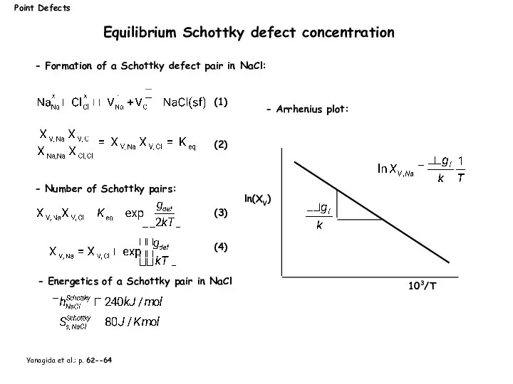
- 12. Point Defects Equilibrium Schottky defect concentration - Number of Schottky pairs: - Formation of a Schottky
- 13. Extrinsic defect concentration I - Total number of cation vacancies: - Substitution of a divalent cation
- 14. Point Defects ln(XV) 103/T XCa=10-4 10-5 10-6 10-4 10-5 10-6 cation vacancies anion vacancies - Temperature
- 15. Point Defects Nonstoichiometric defects In nonstoichiometric defect reactions the composition of the cystal changes as a
- 16. Atomic diffusion is a process whereby the random thermally-activated hopping of atoms in a solid results
- 17. Diffusion Type of diffusion Diffusion paths: HRTEM image of an interface between an aluminum (left) and
- 18. Types of diffusion kinetics: 3 regimes A, B and C are usually distinguished. They are represented
- 19. Diffusion Atomistic diffusion mechanisms Exchange mechanism Ring rotation mechanicsm Vacancy mechanism Interstitial mechanism Diffusion couple t0
- 20. Diffusion Fick’s 1. law dC dx C x The flux J in direction x of the
- 21. Diffusion Fick’s 2. law In regions where the concentration gradient is convex, the flux (and the
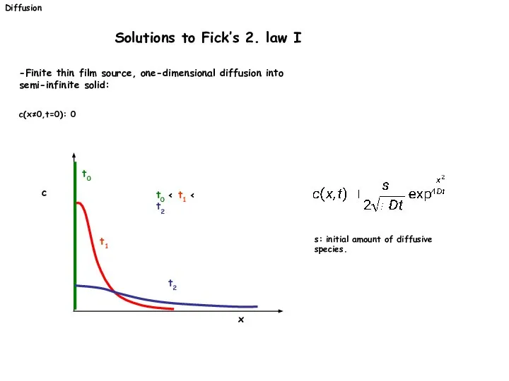
- 22. Diffusion Solutions to Fick’s 2. law I -Finite thin film source, one-dimensional diffusion into semi-infinite solid:
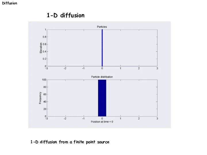
- 23. Diffusion 1-D diffusion 1-D diffusion from a finite point source
- 24. -Finite thin film source of constant concentration, one- dimensional diffusion into semi-infinite solid: c(x≠0,t=0): 0 c(x=0,t):
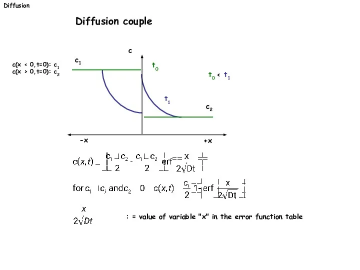
- 25. Diffusion Diffusion couple c(x c(x > 0,t=0): c2 +x -x c t1 t0 t0 c1 c2
- 26. Diffusion 1-D diffusion couple Diffusion profiles for 1-D diffusion couple for different diffusion times
- 27. Diffusion
- 28. - Distance x’ from a source with finite concentration where a certain small amount of the
- 29. Diffusion Diffusion: A thermally activated process I Energy of red atom= ER Minimum energy for jump
- 30. Diffusion Diffusion: A thermally activated process II The preexponential factor and the activation energy for a
- 31. Tracer diffusion coefficients of 18O determined by SIMS profiling for various micro- and nanocrystalline oxides: coarse
- 33. Скачать презентацию
Crystalline solids have a very regular atomic structure: that is, the
Crystalline solids have a very regular atomic structure: that is, the
Point Defects
Point defects in ionic solids I
Frenkel defect: anion vacancy-interstitial
Point Defects
Point defects in ionic solids I
Frenkel defect: anion vacancy-interstitial
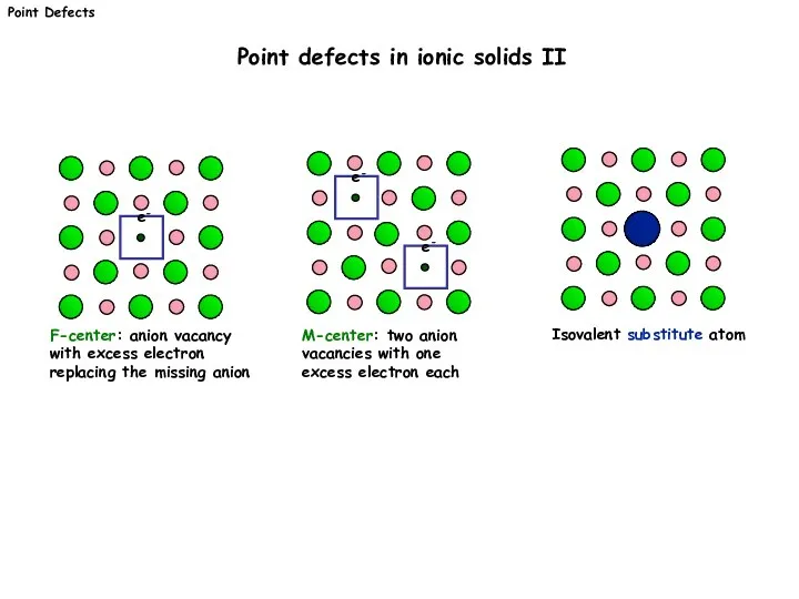
F-center: anion vacancy with excess electron replacing the missing anion
e-
M-center:
F-center: anion vacancy with excess electron replacing the missing anion
e-
M-center:
M corresonds to the species. These include:
atoms - e.g. Si, Ni,
M corresonds to the species. These include:
atoms - e.g. Si, Ni,
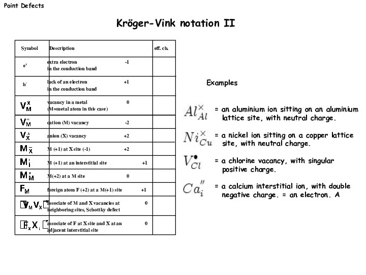
Point Defects
Kröger-Vink notation II
= an aluminium ion sitting on an aluminium
Point Defects
Kröger-Vink notation II
= an aluminium ion sitting on an aluminium
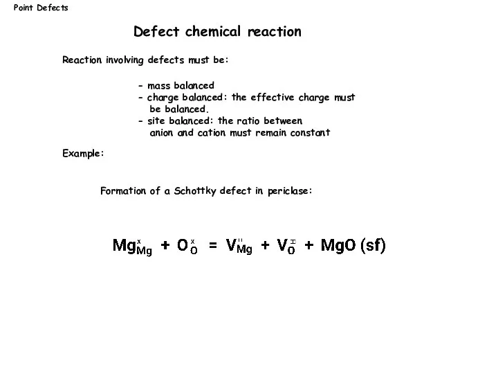
Reaction involving defects must be:
Example:
Point Defects
Defect chemical reaction
Formation of a
Reaction involving defects must be:
Example:
Point Defects
Defect chemical reaction
Formation of a
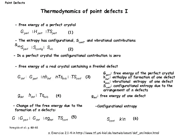
Gperf: free energy of the perfect crystal
hdef: enthalpy of formation
Gperf: free energy of the perfect crystal
hdef: enthalpy of formation
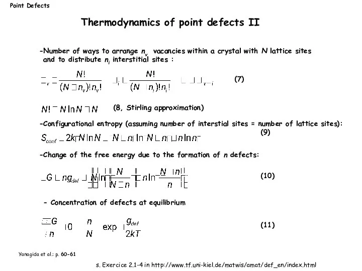
Yanagida et al.: p. 60-61
Number of ways to arrange nv vacancies
Yanagida et al.: p. 60-61
Number of ways to arrange nv vacancies
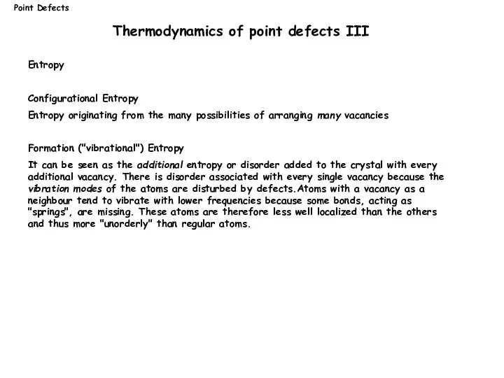
Entropy
Configurational Entropy
Entropy originating from the many possibilities of arranging many vacancies
Formation
Entropy
Configurational Entropy
Entropy originating from the many possibilities of arranging many vacancies
Formation
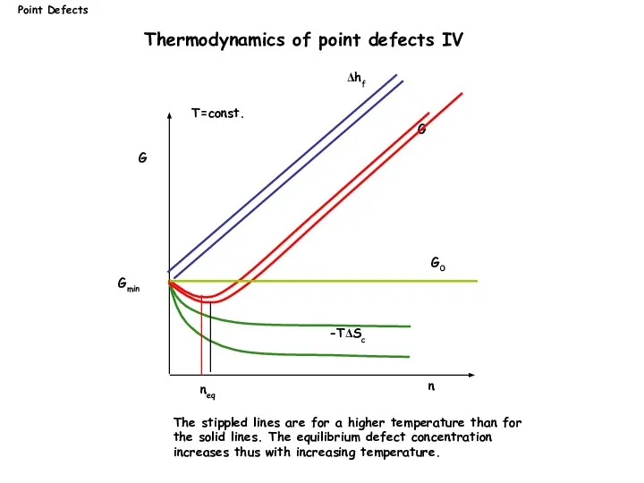
G
n
G0
Δhf
G
neq
-TΔSc
Gmin
T=const.
The stippled lines are for a higher temperature than for the
G
n
G0
Δhf
G
neq
-TΔSc
Gmin
T=const.
The stippled lines are for a higher temperature than for the
Point Defects
Equilibrium Schottky defect concentration
- Number of Schottky pairs:
- Formation
Point Defects
Equilibrium Schottky defect concentration
- Number of Schottky pairs:
- Formation
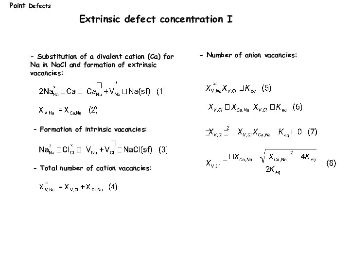
Extrinsic defect concentration I
- Total number of cation vacancies:
- Substitution of
Extrinsic defect concentration I
- Total number of cation vacancies:
- Substitution of
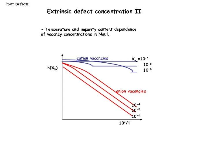
Point Defects
ln(XV)
103/T
XCa=10-4
10-5
10-6
10-4
10-5
10-6
cation vacancies
anion vacancies
- Temperature and impurity content dependence
of vacancy
Point Defects
ln(XV)
103/T
XCa=10-4
10-5
10-6
10-4
10-5
10-6
cation vacancies
anion vacancies
- Temperature and impurity content dependence
of vacancy
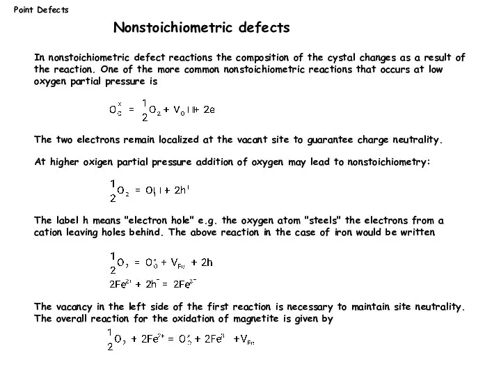
Point Defects
Nonstoichiometric defects
In nonstoichiometric defect reactions the composition of the
Point Defects
Nonstoichiometric defects
In nonstoichiometric defect reactions the composition of the
Atomic diffusion is a process whereby the random thermally-activated hopping of
Atomic diffusion is a process whereby the random thermally-activated hopping of
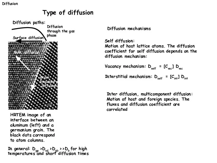
Diffusion
Type of diffusion
Diffusion paths:
HRTEM image of an interface between an
Diffusion
Type of diffusion
Diffusion paths:
HRTEM image of an interface between an
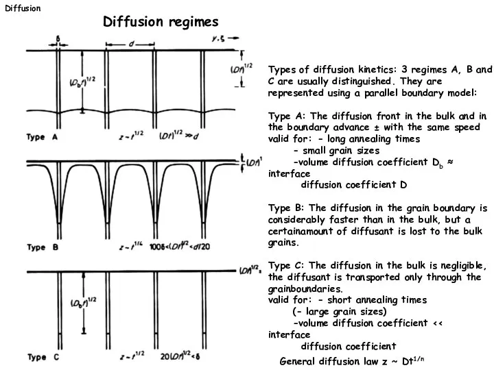
Types of diffusion kinetics: 3 regimes A, B and C are
Types of diffusion kinetics: 3 regimes A, B and C are
Diffusion
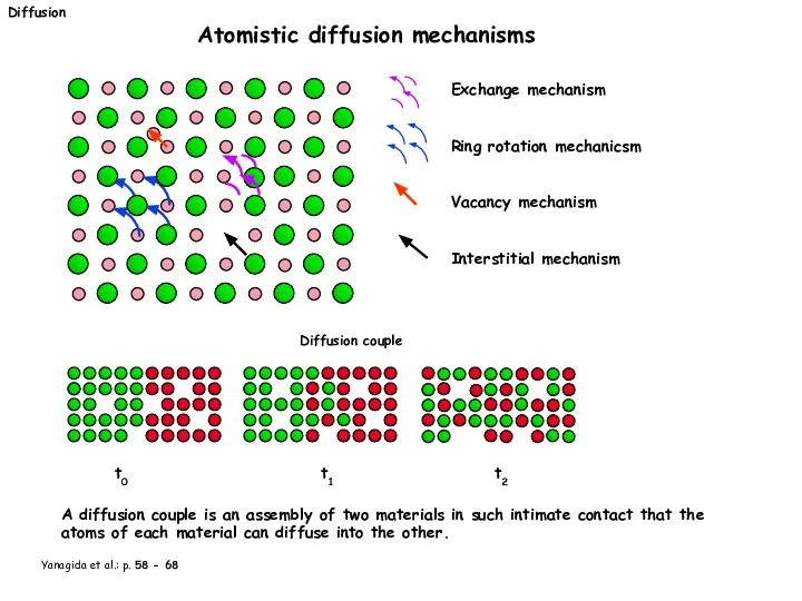
Atomistic diffusion mechanisms
Exchange mechanism
Ring rotation mechanicsm
Vacancy mechanism
Interstitial mechanism
Diffusion couple
t0
Yanagida et
Diffusion
Atomistic diffusion mechanisms
Exchange mechanism
Ring rotation mechanicsm
Vacancy mechanism
Interstitial mechanism
Diffusion couple
t0
Yanagida et
Diffusion
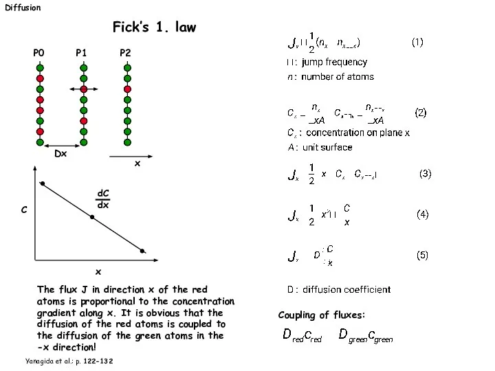
Fick’s 1. law
dC
dx
C
x
The flux J in direction x of the
Diffusion
Fick’s 1. law
dC
dx
C
x
The flux J in direction x of the
Diffusion
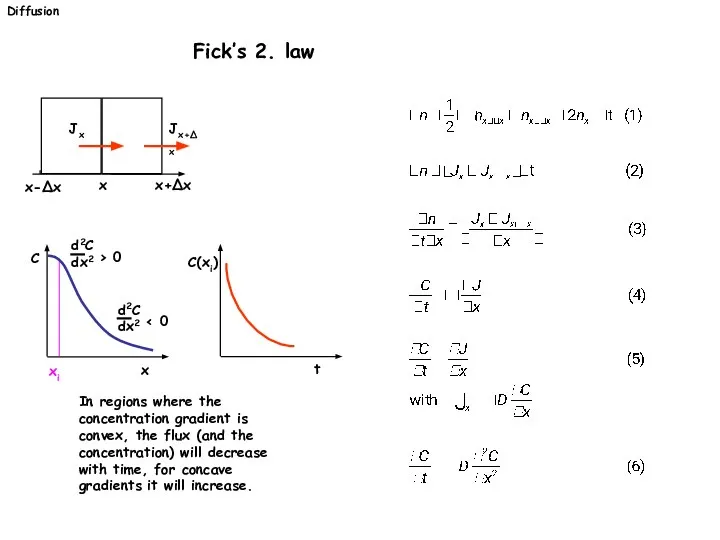
Fick’s 2. law
In regions where the concentration gradient is
Diffusion
Fick’s 2. law
In regions where the concentration gradient is
Diffusion
Solutions to Fick’s 2. law I
-Finite thin film source, one-dimensional
Diffusion
Solutions to Fick’s 2. law I
-Finite thin film source, one-dimensional
Diffusion
1-D diffusion
1-D diffusion from a finite point source
Diffusion
1-D diffusion
1-D diffusion from a finite point source
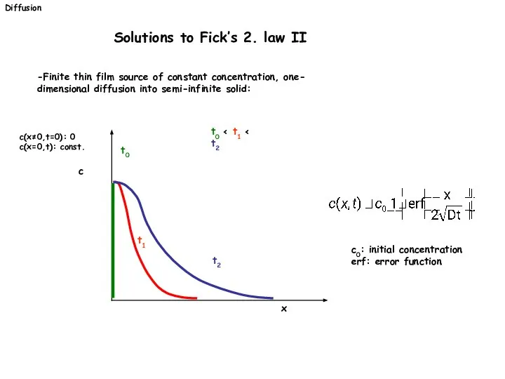
-Finite thin film source of constant concentration, one-
dimensional diffusion into semi-infinite
-Finite thin film source of constant concentration, one-
dimensional diffusion into semi-infinite
Diffusion
Diffusion couple
c(x < 0,t=0): c1
c(x > 0,t=0): c2
+x
-x
c
t1
t0 < t1
Diffusion
Diffusion couple
c(x < 0,t=0): c1
c(x > 0,t=0): c2
+x
-x
c
t1
t0 < t1
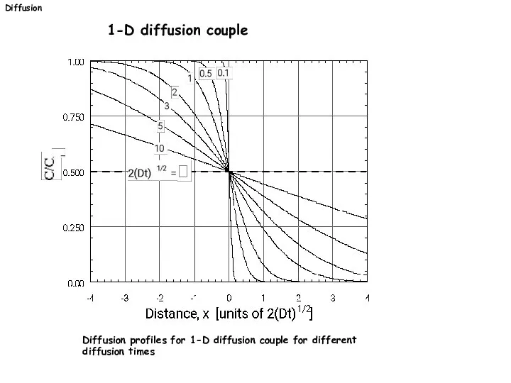
Diffusion
1-D diffusion couple
Diffusion profiles for 1-D diffusion couple for different
Diffusion
1-D diffusion couple
Diffusion profiles for 1-D diffusion couple for different
Diffusion
Diffusion

- Distance x’ from a source with finite concentration where a
- Distance x’ from a source with finite concentration where a
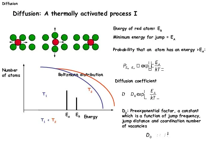
Diffusion
Diffusion: A thermally activated process I
Energy of red atom= ER
Minimum energy
Diffusion
Diffusion: A thermally activated process I
Energy of red atom= ER
Minimum energy
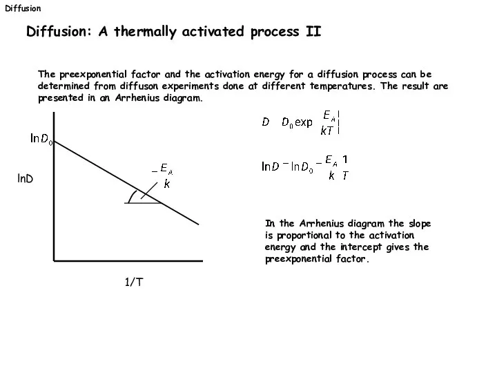
Diffusion
Diffusion: A thermally activated process II
The preexponential factor and the activation
Diffusion
Diffusion: A thermally activated process II
The preexponential factor and the activation
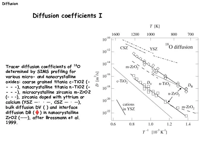
Tracer diffusion coefficients of 18O determined by SIMS profiling for various
Tracer diffusion coefficients of 18O determined by SIMS profiling for various
 Современные положения теории А.М. Бутлерова
 Химические свойства основных классов неорганических соединений
 «Уксусная кислота»
  Исследование минералов в параллельном свете с одним поляризатором
 Биосфера и организм
 Использование углеводородов в медицине
 Хлор
Хлор Коррозия железа
 Расчетная ячейка при МД моделировании. Граничные условия. Элементарная ячейка для атомов аргона
 Model chemistry
 Энергетические эффекты реакций
 Карбоновые кислоты
 Электронное строение атома
 EdExcel Unit C2 – Discovering Chemistry
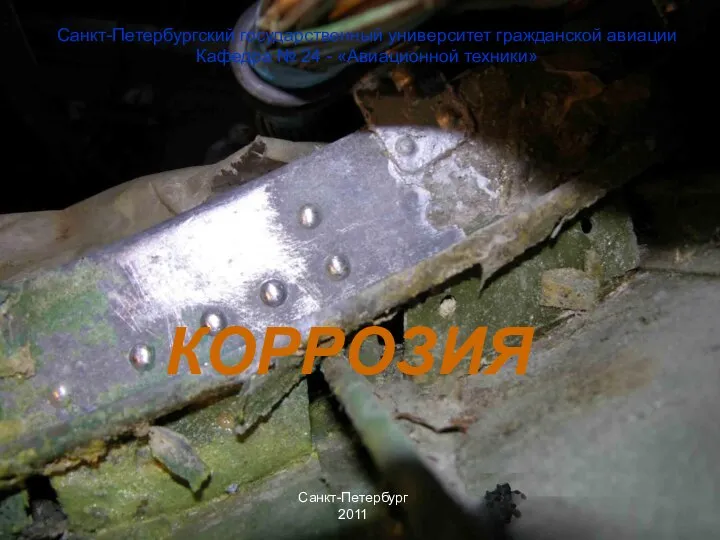 Коррозионные повреждения
 Применение s-, p-, d- элементов в медицине
 Насыщенные углеводороды
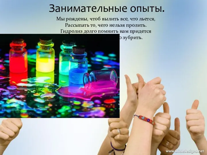 Занимательные опыты
 Количество вещества. Единица измерения вещества моль
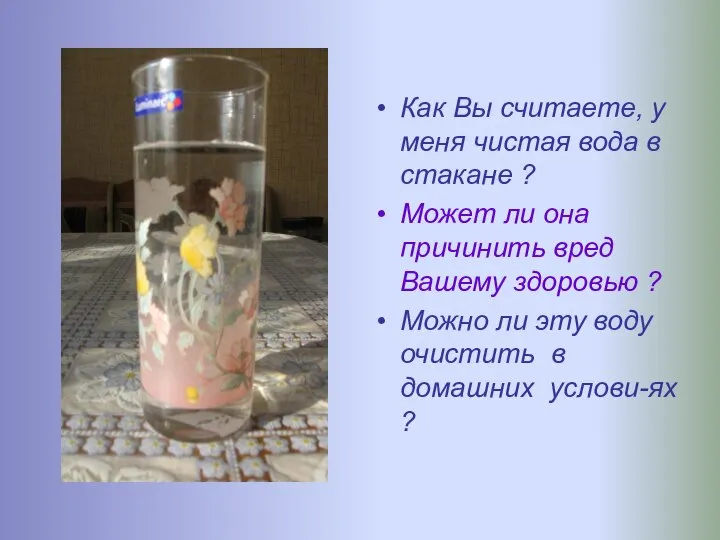 Исследование качества питьевой воды в г. Кашира-8 и способы снижения ее общей жесткости
 Гипергенез и почвообразование
 Азот. Нахождение в природе
 Минералы
 Теоретические основы применения органических реагентов в качественном анализе. (Лекция 8)
 Разложение отходов. 11 класс
 Геохимия рудных месторождений
 Аттестационная работа. Способ формирования метапредметных результатов обучения при обучении химии в условиях реализации ФГОС
 Металлы в природе. Получение и применение металлов