- Основы Python

Содержание
- 2. PIP: PIP Installs Packages sudo pip install packagename sudo pip uninstall packagename cd C:\Python27\Scripts\ pip install
- 3. Arrays – Numerical Python (Numpy) Списки Нет арифметических операций (+, -, *, /, …) Numpy >>>
- 4. Numpy – N-dimensional Array manipulations NumPy – основная библиотека для научных расчетов в Python: поддержка многомерных
- 5. Numpy – Creating vectors From lists numpy.array – создание массива из списка значений >>> import numpy
- 6. >>> import numpy >>> M = numpy.array([[1,2], [3, 4], [5,6], [7,8]], dtype=float) >>> print M [[
- 7. Numpy – Creating matrices >>> L = [[1, 2, 3], [3, 6, 9], [2, 4, 6]]
- 8. Numpy – Matrices use >>> print(a) [[1 2 3] [3 6 9] [2 4 6]] >>>
- 9. Numpy – Creating arrays >>> x = numpy.arange(0, 10, 1) # arguments: start, stop, step >>>
- 10. Numpy – Creating arrays # a diagonal matrix >>> print numpy.diag([1,2,3]) array([[1, 0, 0], [0, 2,
- 11. Numpy – array creation and use >>> d = numpy.arange(5) # just like range() >>> print(d)
- 12. Numpy – array creation and use # random data >>> print numpy.random.rand(5,5) array([[ 0.51531133, 0.74085206, 0.99570623,
- 13. Numpy – Creating arrays Чтение из файла sample.txt: "Stn", "Datum", "Tg", "qTg", "Tn", "qTn", "Tx", "qTx"
- 14. Numpy – Creating arrays Сохранение в файл >>> numpy.savetxt('datasaved.txt', data) datasaved.txt: 1.000000000000000000e+00 1.901010100000000000e+07 -4.900000000000000000e+01 0.000000000000000000e+00 -6.800000000000000000e+01
- 15. Numpy – Creating arrays >>> M = numpy.random.rand(3,3) >>> print M array([[ 0.84188778, 0.70928643, 0.87321035], [
- 16. Numpy – array methods >>> print arr.sum() 145 >>> print arr.mean() 14.5 >>> print arr.std() 2.8722813232690143
- 17. Numpy – array methods - sorting >>> arr = numpy.array([4.5, 2.3, 6.7, 1.2, 1.8, 5.5]) >>>
- 18. Numpy – array functions >>> print arr.sum() 45 >>> print numpy.sum(arr) 45 >>> x = numpy.array([[1,2],[3,4]])
- 19. Numpy – array operations >>> a = numpy.array([[1.0, 2.0], [4.0, 3.0]]) >>> print a [[ 1.
- 20. Numpy – arrays, matrices >>> import numpy >>> m = numpy.mat([[1,2],[3,4]]) >>> a = numpy.array([[1,2],[3,4]]) >>>
- 21. Numpy – matrices >>> a = numpy.array([[1,2],[3,4]]) >>> m = numpy.mat(a) # convert 2-d array to
- 22. >>> a = linspase(0,1,11) >>> print a [ 0. 0.1 0.2 0.3 0.4 0.5 0.6 0.7
- 23. Plotting - matplotlib >>> import matplotlib.pyplot as plt
- 24. Matplotlib.pyplot basic example import matplotlib.pyplot as plt plt.plot([1,3,2,4]) plt.ylabel('some numbers') plt.show()
- 25. Matplotlib.pyplot basic example import numpy import matplotlib.pyplot as plt x = numpy.linspace(0, 5, 10) y =
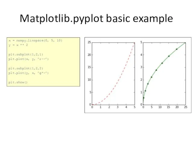
- 27. Matplotlib.pyplot basic example x = numpy.linspace(0, 5, 10) y = x ** 2 plt.subplot(1,2,1) plt.plot(x, y,
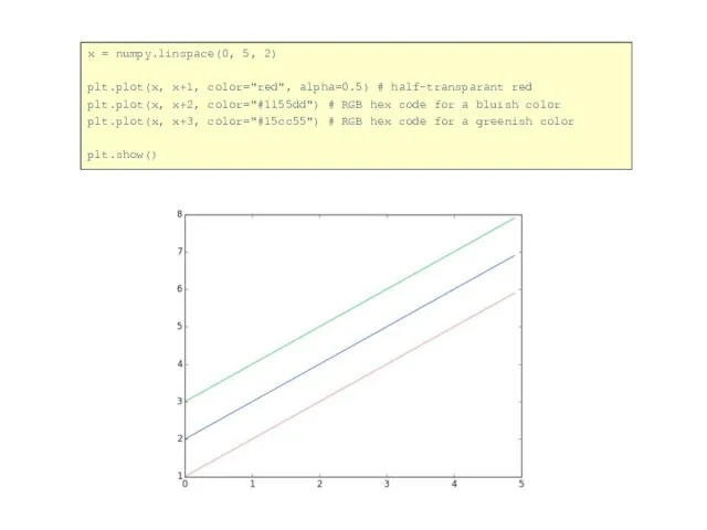
- 28. x = numpy.linspace(0, 5, 2) plt.plot(x, x+1, color="red", alpha=0.5) # half-transparant red plt.plot(x, x+2, color="#1155dd") #
- 29. plt.plot(x, x+1, color="blue", linewidth=0.25) plt.plot(x, x+2, color="blue", linewidth=0.50) plt.plot(x, x+3, color="blue", linewidth=1.00) plt.plot(x, x+4, color="blue", linewidth=2.00)
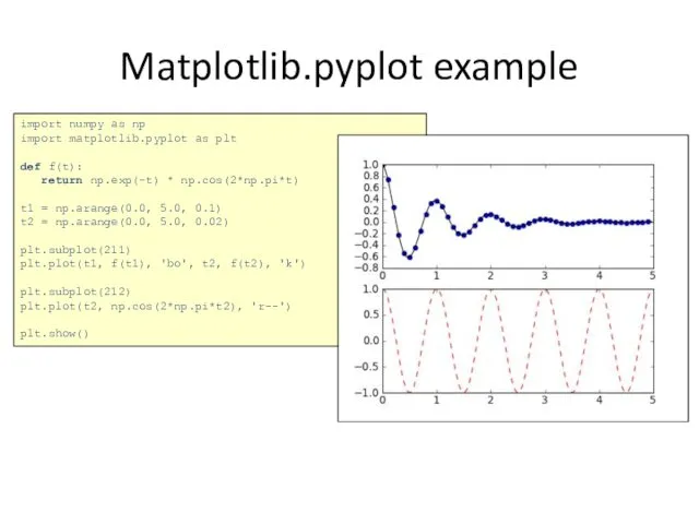
- 30. Matplotlib.pyplot example import numpy as np import matplotlib.pyplot as plt def f(t): return np.exp(-t) * np.cos(2*np.pi*t)
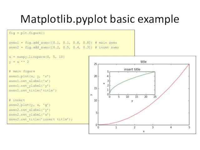
- 31. Matplotlib.pyplot basic example fig = plt.figure() axes1 = fig.add_axes([0.1, 0.1, 0.8, 0.8]) # main axes axes2
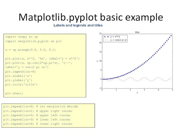
- 32. Matplotlib.pyplot basic example plt.legend(loc=0) # let matplotlib decide plt.legend(loc=1) # upper right corner plt.legend(loc=2) # upper
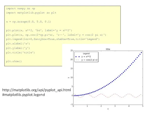
- 33. import numpy as np import matplotlib.pyplot as plt x = np.arange(0.0, 5.0, 0.1) plt.plot(x, x**2, 'bo',
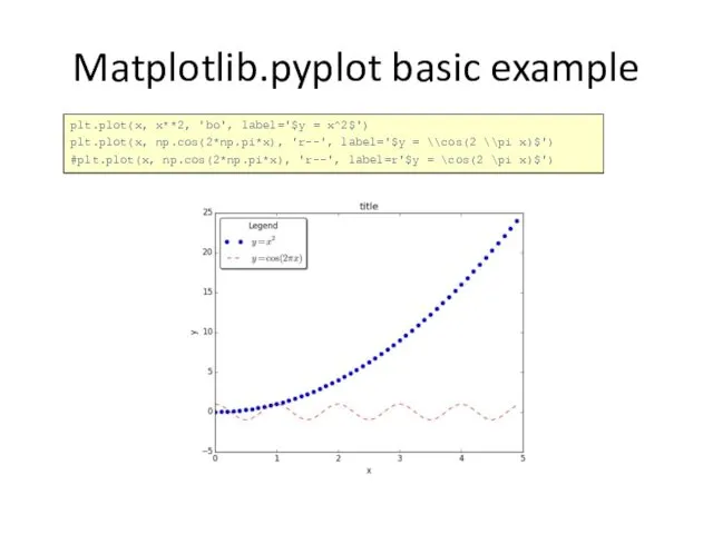
- 34. Matplotlib.pyplot basic example plt.plot(x, x**2, 'bo', label='$y = x^2$') plt.plot(x, np.cos(2*np.pi*x), 'r--', label='$y = \\cos(2 \\pi
- 35. Matplotlib.pyplot basic example x = np.arange(-4.0, 4.0, 0.01) plt.plot(x, x**2, color='blue') plt.xlabel('$x$', fontsize=18) plt.ylabel('$x^2$', color='blue', fontsize=18)
- 36. Overwhelming annotation x = np.arange(-2.0, 2.0, 0.01) plt.plot(x, np.cos(2*np.pi*x)) plt.xlim(-2.1, 2.1) plt.ylim(-1.5, 1.5) plt.annotate('-', xy=(-2,1), xytext=(-1.8,1.3),
- 37. Matplotlib.pyplot basic example x = np.linspace(-1.0, 2.0, 16) plt.subplot(221) plt.scatter(x, np.sin(50 * x + 12)) plt.subplot(222)
- 38. Matplotlib.pyplot basic example import matplotlib.pyplot as plt import pyfits data = pyfits.getdata('frame-g-006073-4-0063.fits') plt.imshow(data, cmap='gnuplot2') plt.colorbar() plt.show()
- 40. # plt.show() plt.savefig('filename', orientation='landscape', format='eps') # orientation='portrait' # 'landscape‘ # format='png'(по умолчанию) # 'pdf' # 'eps'
- 41. Пакет SciPy
- 42. Генерация и визуализация случайных последовательностей Субмодуль numpy.random включает векторные версии нескольких различных генераторов случайных чисел. >>>
- 43. Data Modeling and Fitting curve_fit – метод, позволяющий аппроксимировать набор точек некоторой функциональной зависимостью, основанный на
- 44. Data Modeling and Fitting curve_fit – метод, позволяющий аппроксимировать набор точек некоторой функциональной зависимомтью, основанный на
- 45. функция fsolve – решение уравнений >>> import numpy as np >>> from scipy.optimize import fsolve >>>
- 46. Interpolation >>> import matplotlib.pyplot as plt >>> import numpy as np >>> from scipy.interpolate import interp1d
- 47. Интегрирование >>> from scipy.integrate import * [ , ] = quad(f(x),xmin,xmax) inf изображает бесконечный предел интегрирования
- 48. Интегрирование >>> import numpy as np >>> from scipy.integrate import * >>> x=np.linspace(0,np.pi,10) >>> f =
- 49. Решение дифференциальных уравнений Функция odeint odeint(f(x,t),x0, )
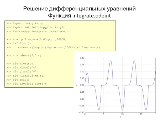
- 50. Решение дифференциальных уравнений Функция integrate.odeint >>> import numpy as np >>> import matplotlib.pyplot as plt >>>
- 51. Решение дифференциальных уравнений Функция integrate.odeint
- 52. Решение дифференциальных уравнений Функция integrate.odeint >>> import numpy as np >>> import matplotlib.pyplot as plt >>>
- 53. На языке программирования Python для спектра звезды, полученного при наблюдениях в оптическом диапазоне (spec_star.txt), определить температуру
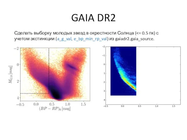
- 54. GAIA DR2 http://gea.esac.esa.int/archive/ Сделать выборку звезд в окрестности Солнца ( parallax_over_error >= 5 M_G BP-RP parallax
- 56. Сделать выборку молодых звезд в окрестности Солнца ( GAIA DR2
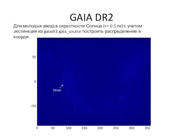
- 57. GAIA DR2 Для молодых звезд в окрестности Солнца (
- 59. Скачать презентацию
PIP: PIP Installs Packages
sudo pip install packagename
sudo pip uninstall packagename
cd C:\Python27\Scripts\
pip
PIP: PIP Installs Packages
sudo pip install packagename
sudo pip uninstall packagename
cd C:\Python27\Scripts\
pip
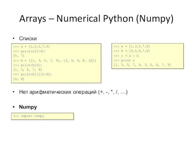
Arrays – Numerical Python (Numpy)
Списки
Нет арифметических операций (+, -, *, /,
Arrays – Numerical Python (Numpy)
Списки
Нет арифметических операций (+, -, *, /,
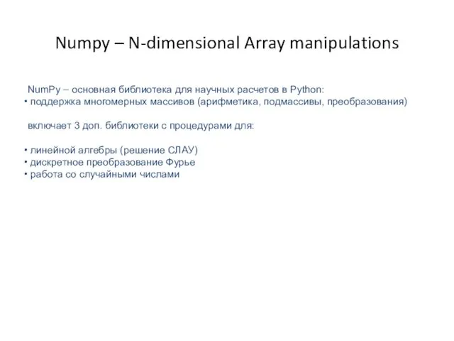
Numpy – N-dimensional Array manipulations
NumPy – основная библиотека для научных расчетов
Numpy – N-dimensional Array manipulations
NumPy – основная библиотека для научных расчетов
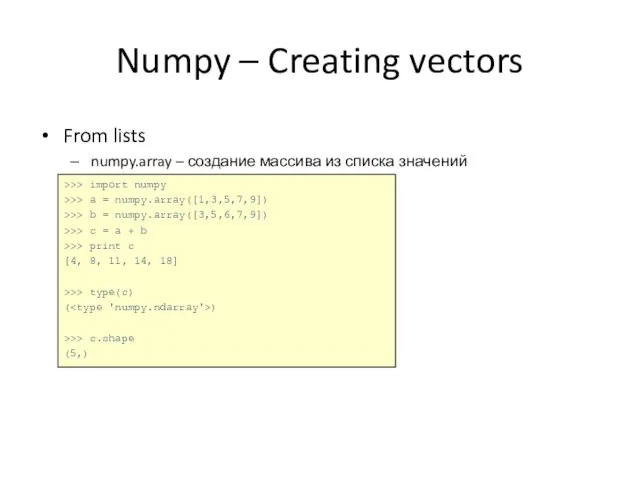
Numpy – Creating vectors
From lists
numpy.array – создание массива из списка значений
>>>
Numpy – Creating vectors
From lists
numpy.array – создание массива из списка значений
>>>
![>>> import numpy >>> M = numpy.array([[1,2], [3, 4], [5,6], [7,8]],](/_ipx/f_webp&q_80&fit_contain&s_1440x1080/imagesDir/jpg/454592/slide-5.jpg)
>>> import numpy
>>> M = numpy.array([[1,2], [3, 4], [5,6], [7,8]], dtype=float)
>>>
>>> import numpy
>>> M = numpy.array([[1,2], [3, 4], [5,6], [7,8]], dtype=float)
>>>
![Numpy – Creating matrices >>> L = [[1, 2, 3], [3,](/_ipx/f_webp&q_80&fit_contain&s_1440x1080/imagesDir/jpg/454592/slide-6.jpg)
Numpy – Creating matrices
>>> L = [[1, 2, 3], [3, 6,
Numpy – Creating matrices
>>> L = [[1, 2, 3], [3, 6,
![Numpy – Matrices use >>> print(a) [[1 2 3] [3 6](/_ipx/f_webp&q_80&fit_contain&s_1440x1080/imagesDir/jpg/454592/slide-7.jpg)
Numpy – Matrices use
>>> print(a)
[[1 2 3]
[3 6
Numpy – Matrices use
>>> print(a)
[[1 2 3]
[3 6
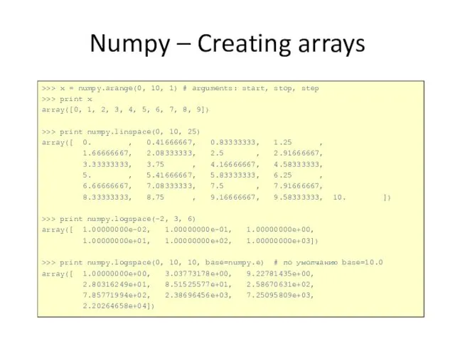
Numpy – Creating arrays
>>> x = numpy.arange(0, 10, 1) # arguments:
Numpy – Creating arrays
>>> x = numpy.arange(0, 10, 1) # arguments:
![Numpy – Creating arrays # a diagonal matrix >>> print numpy.diag([1,2,3])](/_ipx/f_webp&q_80&fit_contain&s_1440x1080/imagesDir/jpg/454592/slide-9.jpg)
Numpy – Creating arrays
# a diagonal matrix
>>> print numpy.diag([1,2,3])
array([[1, 0, 0],
Numpy – Creating arrays
# a diagonal matrix
>>> print numpy.diag([1,2,3])
array([[1, 0, 0],
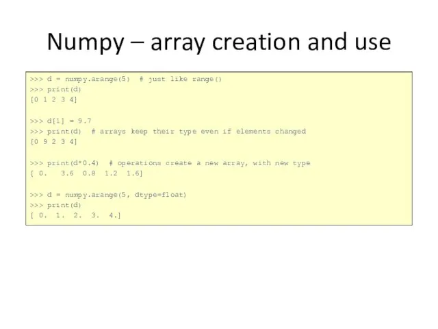
Numpy – array creation and use
>>> d = numpy.arange(5) # just
Numpy – array creation and use
>>> d = numpy.arange(5) # just
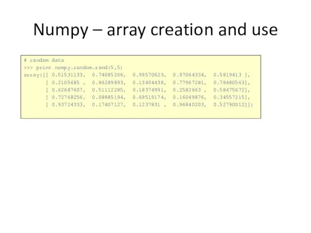
Numpy – array creation and use
# random data
>>> print numpy.random.rand(5,5)
array([[ 0.51531133,
Numpy – array creation and use
# random data
>>> print numpy.random.rand(5,5)
array([[ 0.51531133,
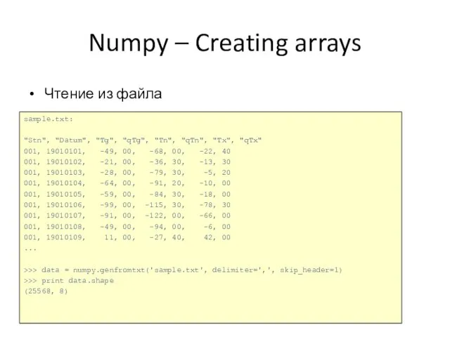
Numpy – Creating arrays
Чтение из файла
sample.txt:
"Stn", "Datum", "Tg", "qTg", "Tn", "qTn",
Numpy – Creating arrays
Чтение из файла
sample.txt:
"Stn", "Datum", "Tg", "qTg", "Tn", "qTn",
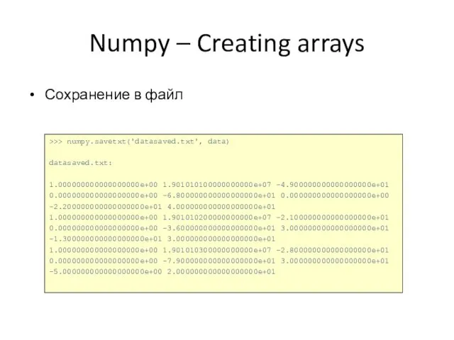
Numpy – Creating arrays
Сохранение в файл
>>> numpy.savetxt('datasaved.txt', data)
datasaved.txt:
1.000000000000000000e+00 1.901010100000000000e+07 -4.900000000000000000e+01 0.000000000000000000e+00
Numpy – Creating arrays
Сохранение в файл
>>> numpy.savetxt('datasaved.txt', data)
datasaved.txt:
1.000000000000000000e+00 1.901010100000000000e+07 -4.900000000000000000e+01 0.000000000000000000e+00
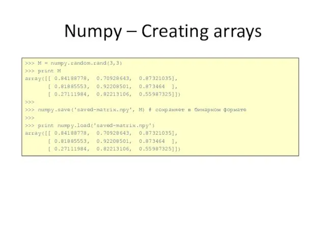
Numpy – Creating arrays
>>> M = numpy.random.rand(3,3)
>>> print M
array([[ 0.84188778, 0.70928643,
Numpy – Creating arrays
>>> M = numpy.random.rand(3,3)
>>> print M
array([[ 0.84188778, 0.70928643,
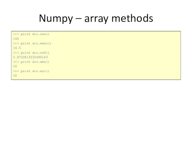
Numpy – array methods
>>> print arr.sum()
145
>>> print arr.mean()
14.5
Numpy – array methods
>>> print arr.sum()
145
>>> print arr.mean()
14.5
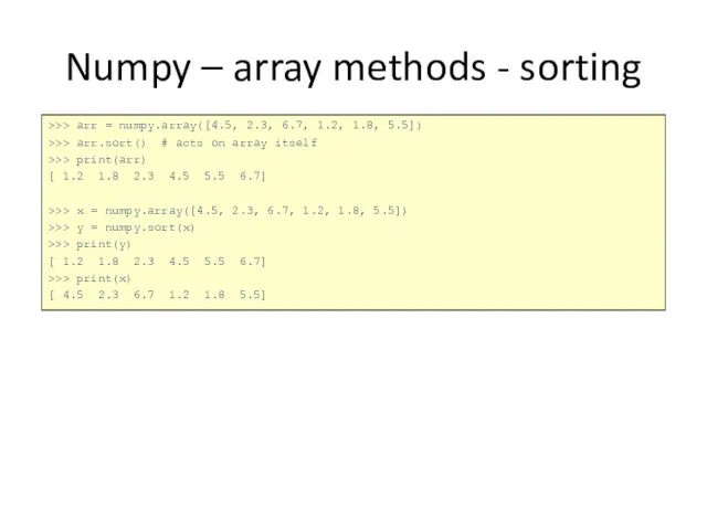
Numpy – array methods - sorting
>>> arr = numpy.array([4.5, 2.3, 6.7,
Numpy – array methods - sorting
>>> arr = numpy.array([4.5, 2.3, 6.7,
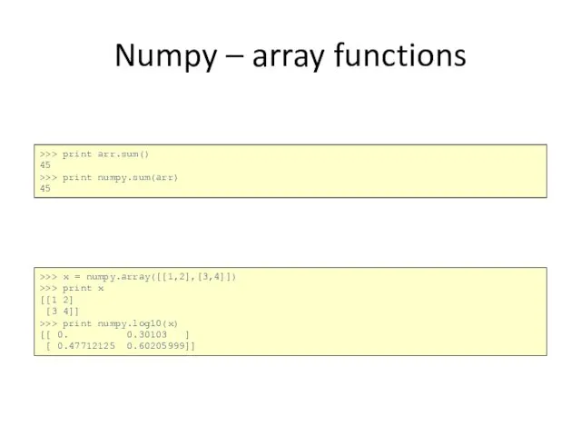
Numpy – array functions
>>> print arr.sum()
45
>>> print numpy.sum(arr)
45
>>>
Numpy – array functions
>>> print arr.sum()
45
>>> print numpy.sum(arr)
45
>>>
![Numpy – array operations >>> a = numpy.array([[1.0, 2.0], [4.0, 3.0]])](/_ipx/f_webp&q_80&fit_contain&s_1440x1080/imagesDir/jpg/454592/slide-18.jpg)
Numpy – array operations
>>> a = numpy.array([[1.0, 2.0], [4.0, 3.0]])
>>>
Numpy – array operations
>>> a = numpy.array([[1.0, 2.0], [4.0, 3.0]])
>>>
![Numpy – arrays, matrices >>> import numpy >>> m = numpy.mat([[1,2],[3,4]])](/_ipx/f_webp&q_80&fit_contain&s_1440x1080/imagesDir/jpg/454592/slide-19.jpg)
Numpy – arrays, matrices
>>> import numpy
>>> m = numpy.mat([[1,2],[3,4]])
>>>
Numpy – arrays, matrices
>>> import numpy
>>> m = numpy.mat([[1,2],[3,4]])
>>>
![Numpy – matrices >>> a = numpy.array([[1,2],[3,4]]) >>> m = numpy.mat(a)](/_ipx/f_webp&q_80&fit_contain&s_1440x1080/imagesDir/jpg/454592/slide-20.jpg)
Numpy – matrices
>>> a = numpy.array([[1,2],[3,4]])
>>> m = numpy.mat(a) #
Numpy – matrices
>>> a = numpy.array([[1,2],[3,4]])
>>> m = numpy.mat(a) #
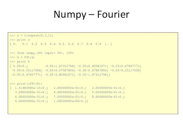
>>> a = linspase(0,1,11)
>>> print a
[ 0. 0.1 0.2 0.3
>>> a = linspase(0,1,11)
>>> print a
[ 0. 0.1 0.2 0.3
Plotting - matplotlib
>>> import matplotlib.pyplot as plt
Plotting - matplotlib
>>> import matplotlib.pyplot as plt
![Matplotlib.pyplot basic example import matplotlib.pyplot as plt plt.plot([1,3,2,4]) plt.ylabel('some numbers') plt.show()](/_ipx/f_webp&q_80&fit_contain&s_1440x1080/imagesDir/jpg/454592/slide-23.jpg)
Matplotlib.pyplot basic example
import matplotlib.pyplot as plt plt.plot([1,3,2,4])
plt.ylabel('some numbers')
plt.show()
Matplotlib.pyplot basic example
import matplotlib.pyplot as plt plt.plot([1,3,2,4])
plt.ylabel('some numbers')
plt.show()
Matplotlib.pyplot basic example
import numpy
import matplotlib.pyplot as plt
x = numpy.linspace(0, 5, 10)
y
Matplotlib.pyplot basic example
import numpy
import matplotlib.pyplot as plt
x = numpy.linspace(0, 5, 10)
y

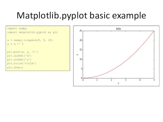
Matplotlib.pyplot basic example
x = numpy.linspace(0, 5, 10)
y = x ** 2
plt.subplot(1,2,1)
plt.plot(x,
Matplotlib.pyplot basic example
x = numpy.linspace(0, 5, 10)
y = x ** 2
plt.subplot(1,2,1)
plt.plot(x,
x = numpy.linspace(0, 5, 2)
plt.plot(x, x+1, color="red", alpha=0.5) # half-transparant red
plt.plot(x,
x = numpy.linspace(0, 5, 2)
plt.plot(x, x+1, color="red", alpha=0.5) # half-transparant red
plt.plot(x,
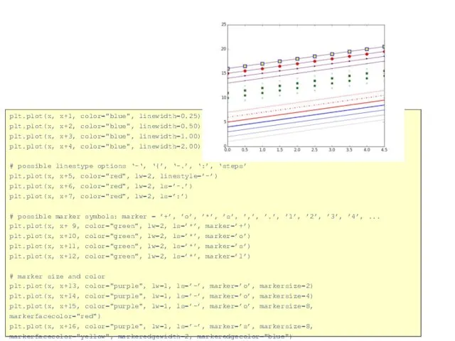
plt.plot(x, x+1, color="blue", linewidth=0.25)
plt.plot(x, x+2, color="blue", linewidth=0.50)
plt.plot(x, x+3, color="blue", linewidth=1.00)
plt.plot(x, x+4,
plt.plot(x, x+1, color="blue", linewidth=0.25)
plt.plot(x, x+2, color="blue", linewidth=0.50)
plt.plot(x, x+3, color="blue", linewidth=1.00)
plt.plot(x, x+4,
Matplotlib.pyplot example
import numpy as np
import matplotlib.pyplot as plt
def f(t):
Matplotlib.pyplot example
import numpy as np
import matplotlib.pyplot as plt
def f(t):
Matplotlib.pyplot basic example
fig = plt.figure()
axes1 = fig.add_axes([0.1, 0.1, 0.8, 0.8]) #
Matplotlib.pyplot basic example
fig = plt.figure()
axes1 = fig.add_axes([0.1, 0.1, 0.8, 0.8]) #
Matplotlib.pyplot basic example
plt.legend(loc=0) # let matplotlib decide plt.legend(loc=1) # upper right
Matplotlib.pyplot basic example
plt.legend(loc=0) # let matplotlib decide plt.legend(loc=1) # upper right
import numpy as np
import matplotlib.pyplot as plt
x = np.arange(0.0, 5.0, 0.1)
plt.plot(x,
import numpy as np
import matplotlib.pyplot as plt
x = np.arange(0.0, 5.0, 0.1)
plt.plot(x,
Matplotlib.pyplot basic example
plt.plot(x, x**2, 'bo', label='$y = x^2$')
plt.plot(x, np.cos(2*np.pi*x), 'r--', label='$y
Matplotlib.pyplot basic example
plt.plot(x, x**2, 'bo', label='$y = x^2$')
plt.plot(x, np.cos(2*np.pi*x), 'r--', label='$y
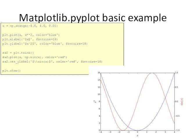
Matplotlib.pyplot basic example
x = np.arange(-4.0, 4.0, 0.01)
plt.plot(x, x**2, color='blue')
plt.xlabel('$x$', fontsize=18)
plt.ylabel('$x^2$', color='blue',
Matplotlib.pyplot basic example
x = np.arange(-4.0, 4.0, 0.01)
plt.plot(x, x**2, color='blue')
plt.xlabel('$x$', fontsize=18)
plt.ylabel('$x^2$', color='blue',
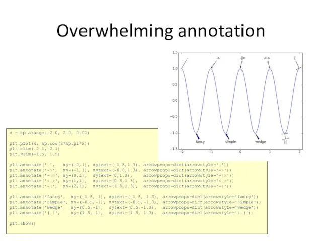
Overwhelming annotation
x = np.arange(-2.0, 2.0, 0.01)
plt.plot(x, np.cos(2*np.pi*x))
plt.xlim(-2.1, 2.1)
plt.ylim(-1.5, 1.5)
plt.annotate('-', xy=(-2,1), xytext=(-1.8,1.3),
Overwhelming annotation
x = np.arange(-2.0, 2.0, 0.01)
plt.plot(x, np.cos(2*np.pi*x))
plt.xlim(-2.1, 2.1)
plt.ylim(-1.5, 1.5)
plt.annotate('-', xy=(-2,1), xytext=(-1.8,1.3),
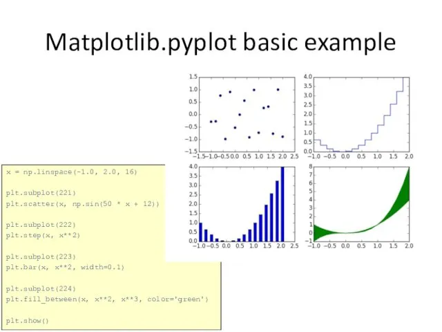
Matplotlib.pyplot basic example
x = np.linspace(-1.0, 2.0, 16)
plt.subplot(221)
plt.scatter(x, np.sin(50 * x +
Matplotlib.pyplot basic example
x = np.linspace(-1.0, 2.0, 16)
plt.subplot(221)
plt.scatter(x, np.sin(50 * x +

Matplotlib.pyplot basic example
import matplotlib.pyplot as plt
import pyfits
data = pyfits.getdata('frame-g-006073-4-0063.fits')
plt.imshow(data, cmap='gnuplot2')
plt.colorbar()
plt.show()
Matplotlib.pyplot basic example
import matplotlib.pyplot as plt
import pyfits
data = pyfits.getdata('frame-g-006073-4-0063.fits')
plt.imshow(data, cmap='gnuplot2')
plt.colorbar()
plt.show()

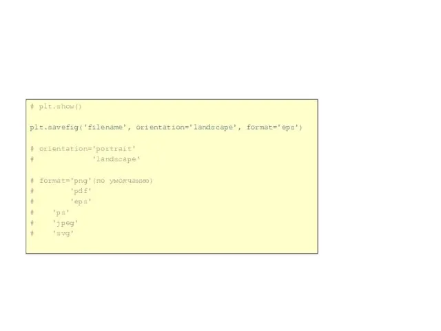
# plt.show()
plt.savefig('filename', orientation='landscape', format='eps')
# orientation='portrait'
# 'landscape‘
# format='png'(по умолчанию)
# 'pdf'
# 'eps'
# 'ps'
#
# plt.show()
plt.savefig('filename', orientation='landscape', format='eps')
# orientation='portrait'
# 'landscape‘
# format='png'(по умолчанию)
# 'pdf'
# 'eps'
# 'ps'
#

Пакет SciPy
Пакет SciPy
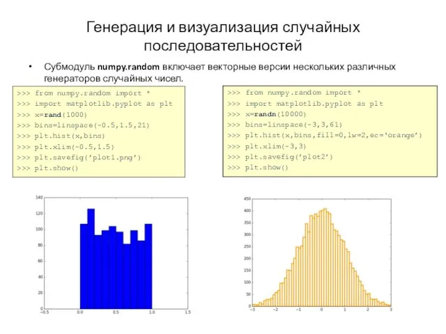
Генерация и визуализация случайных последовательностей
Субмодуль numpy.random включает векторные версии нескольких различных
Генерация и визуализация случайных последовательностей
Субмодуль numpy.random включает векторные версии нескольких различных
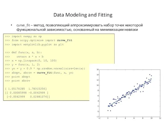
Data Modeling and Fitting
curve_fit – метод, позволяющий аппроксимировать набор точек некоторой
Data Modeling and Fitting
curve_fit – метод, позволяющий аппроксимировать набор точек некоторой
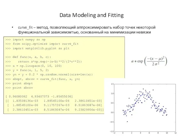
Data Modeling and Fitting
curve_fit – метод, позволяющий аппроксимировать набор точек некоторой
Data Modeling and Fitting
curve_fit – метод, позволяющий аппроксимировать набор точек некоторой
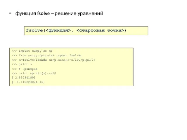
функция fsolve – решение уравнений
>>> import numpy as np
>>> from scipy.optimize
функция fsolve – решение уравнений
>>> import numpy as np
>>> from scipy.optimize
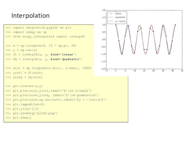
Interpolation
>>> import matplotlib.pyplot as plt
>>> import numpy as np
>>> from scipy.interpolate
Interpolation
>>> import matplotlib.pyplot as plt
>>> import numpy as np
>>> from scipy.interpolate
![Интегрирование >>> from scipy.integrate import * [ , ] = quad(f(x),xmin,xmax)](/_ipx/f_webp&q_80&fit_contain&s_1440x1080/imagesDir/jpg/454592/slide-46.jpg)
Интегрирование
>>> from scipy.integrate import *
[<интеграл>,<ошибка>] = quad(f(x),xmin,xmax)
inf изображает бесконечный предел интегрирования
Субмодуль
Интегрирование
>>> from scipy.integrate import *
[<интеграл>,<ошибка>] = quad(f(x),xmin,xmax)
inf изображает бесконечный предел интегрирования
Субмодуль
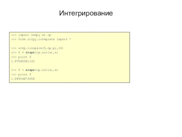
Интегрирование
>>> import numpy as np
>>> from scipy.integrate import *
>>> x=np.linspace(0,np.pi,10)
>>> f
Интегрирование
>>> import numpy as np
>>> from scipy.integrate import *
>>> x=np.linspace(0,np.pi,10)
>>> f
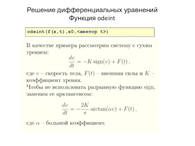
Решение дифференциальных уравнений
Функция odeint
odeint(f(x,t),x0,<вектор t>)
Решение дифференциальных уравнений
Функция odeint
odeint(f(x,t),x0,<вектор t>)
Решение дифференциальных уравнений
Функция integrate.odeint
>>> import numpy as np
>>> import matplotlib.pyplot as
Решение дифференциальных уравнений
Функция integrate.odeint
>>> import numpy as np
>>> import matplotlib.pyplot as
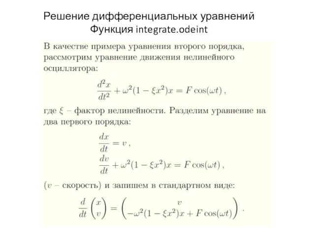
Решение дифференциальных уравнений
Функция integrate.odeint
Решение дифференциальных уравнений
Функция integrate.odeint
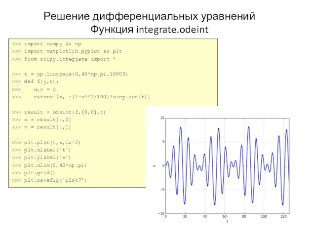
Решение дифференциальных уравнений
Функция integrate.odeint
>>> import numpy as np
>>> import matplotlib.pyplot as
Решение дифференциальных уравнений
Функция integrate.odeint
>>> import numpy as np
>>> import matplotlib.pyplot as
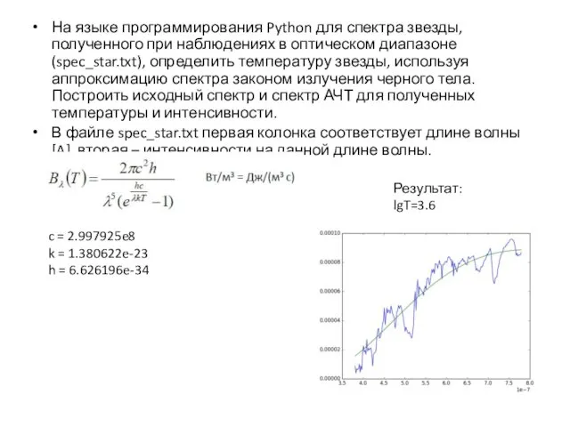
На языке программирования Python для спектра звезды, полученного при наблюдениях в
На языке программирования Python для спектра звезды, полученного при наблюдениях в
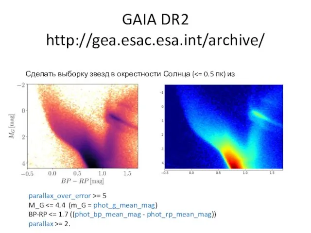
GAIA DR2 http://gea.esac.esa.int/archive/
Сделать выборку звезд в окрестности Солнца (<= 0.5 пк)
GAIA DR2 http://gea.esac.esa.int/archive/
Сделать выборку звезд в окрестности Солнца (<= 0.5 пк)

Сделать выборку молодых звезд в окрестности Солнца (<= 0.5 пк) с
Сделать выборку молодых звезд в окрестности Солнца (<= 0.5 пк) с
GAIA DR2
Для молодых звезд в окрестности Солнца (<= 0.5 пк) с
GAIA DR2
Для молодых звезд в окрестности Солнца (<= 0.5 пк) с
 Microcontrollers misis 2017
 Программирование на языке Java. Тема 11. Логический тип данных
 SmartReport для сети ресторанов
 Креативное программирование. Scratch 3
 Мова HTML
 Информационные системы
 Юзабилити интернет-магазинов: Что не видят продавцы и покупатели Владимир Ямин Группа юзабилити-экспертов 1point (www.1point.ru)
 Алгоритм и его формальное исполнение
 ЭЦП
ЭЦП Многомерные массивы. Занятие 9
 Модели и их типы
 Объекты и их имена. 5-7 класс
 Теория информации
 Источники и приемники информации. (3 класс)
 Организация, принципы построения и функционирования компьютерных сетей. 2-курс. Занятие 02, 03
 Презентация "Аналогия и закономерность" - скачать презентации по Информатике
 Проект Новый информационный канал
 Множественные базы данных
 Разработка приложения Квест с использованием веб-технологии
 Задания по информатике. 4 класс
 Язык программирования JAVA. Функции
 Программы работы с текстом. Текстовые процессоры
 Сортировка, удаление и добавление записей
 Файлы. Файловая структура внешней памяти
 Автоматизированные информационно-управляющие системы
 Помощь к практическому заданию 12 по информатике. Фильтр
 Шаблон презинтации
 Создание формул Использование редактора формул Microsoft Equation