- Probability Random Variables Preparatory Notes

Содержание
- 2. Overview Basic Probability Discrete Random Variables Continuous Random Variables Concepts Laws and Notation Conditional Probability Total
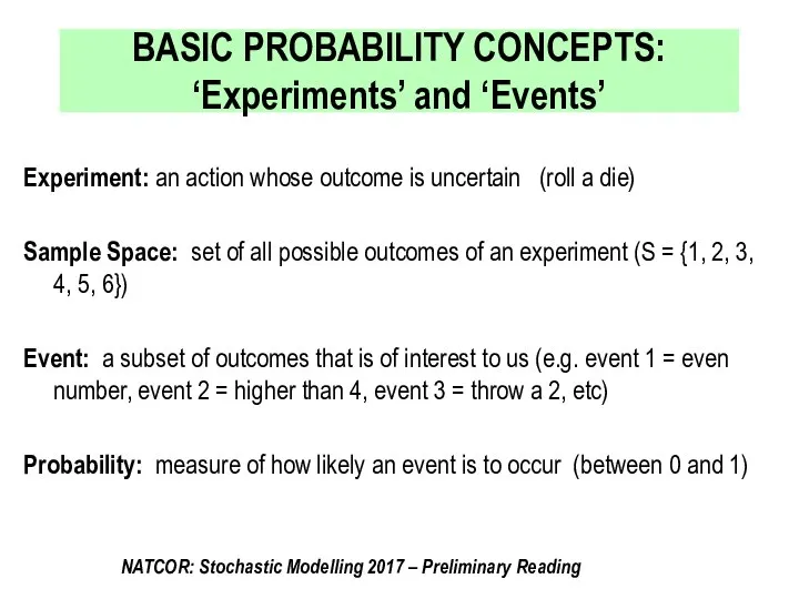
- 3. BASIC PROBABILITY CONCEPTS: ‘Experiments’ and ‘Events’ Experiment: an action whose outcome is uncertain (roll a die)
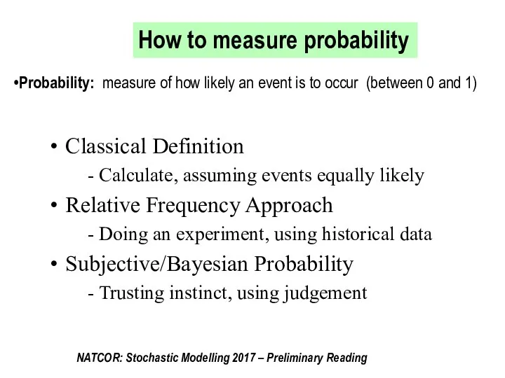
- 4. How to measure probability Probability: measure of how likely an event is to occur (between 0
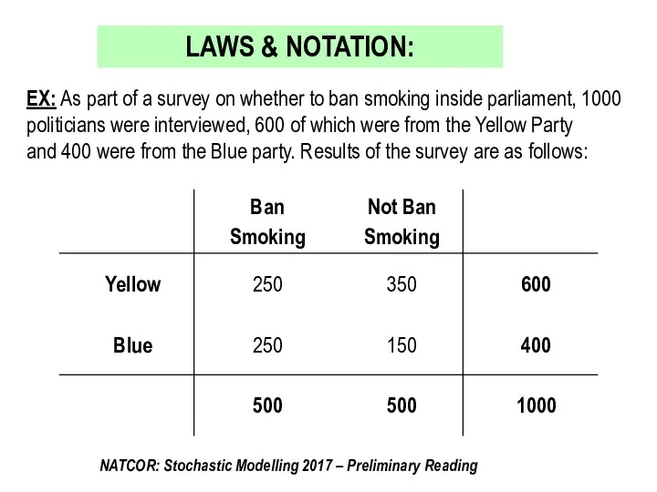
- 5. EX: As part of a survey on whether to ban smoking inside parliament, 1000 politicians were
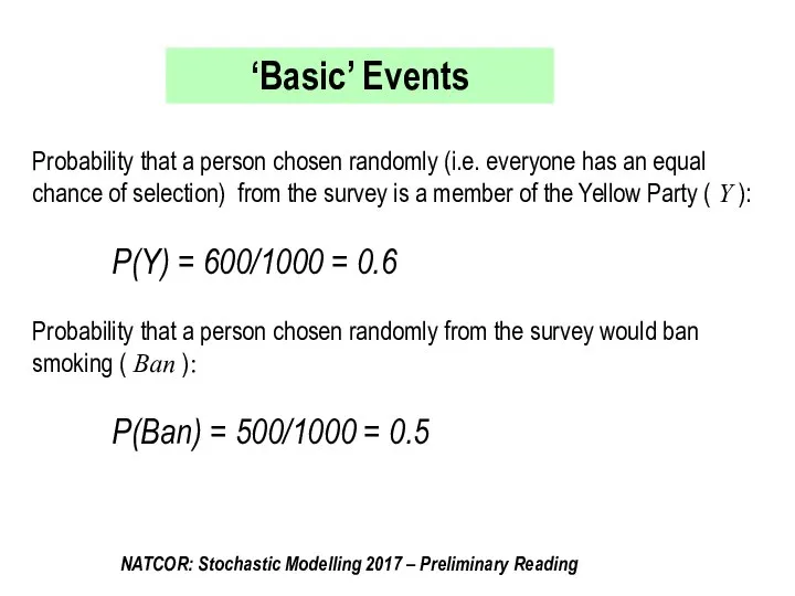
- 6. Probability that a person chosen randomly (i.e. everyone has an equal chance of selection) from the
- 7. Probability that a person chosen randomly from the survey is a member of the Yellow Party
- 8. Probability that a person chosen is either from the Yellow Party ( Y ) or would
- 9. Addition Law for Probabilities (in general): A special case is when Events A and B are
- 10. The Conditional Probability that a randomly chosen person would ban smoking ( Ban ) given that
- 11. Multiplication Law for Probabilities (in general) or A special case is when Events A and B
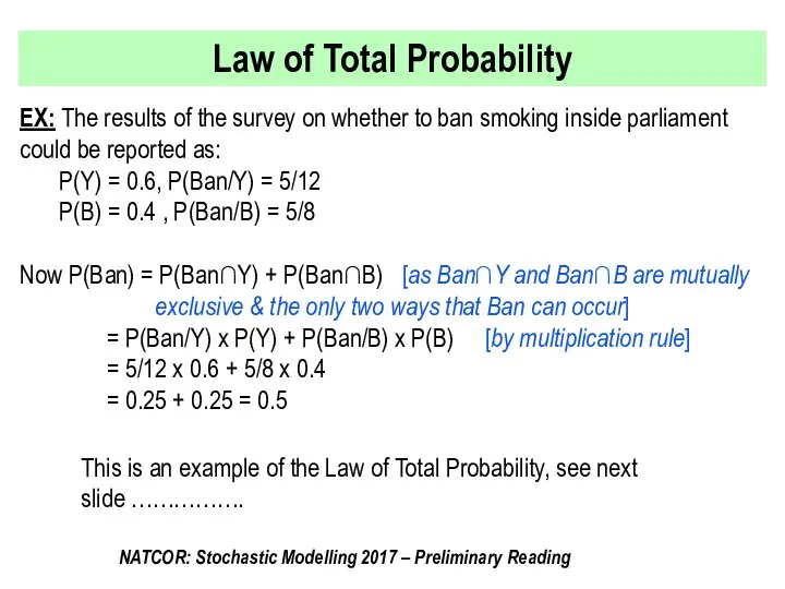
- 12. Law of Total Probability EX: The results of the survey on whether to ban smoking inside
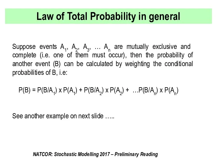
- 13. Law of Total Probability in general Suppose events A1, A2, A3, … An are mutually exclusive
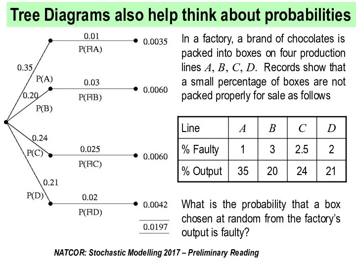
- 14. Tree Diagrams also help think about probabilities In a factory, a brand of chocolates is packed
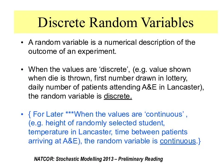
- 15. Discrete Random Variables A random variable is a numerical description of the outcome of an experiment.
- 16. Probability Mass Function (pmf) of a discrete random variable The pmf, p(x), of a discrete random
- 17. Expected value and variance of discrete random variables The expected value, or mean, of a discrete
- 18. E.g. Sum of values when two dice are thrown:
- 19. Expected value and variance of combinations of discrete random variables If X and Y are random
- 20. Law of Total Probability for Expected Values of a discrete random variable Suppose events A1, A2,
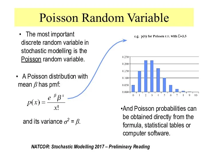
- 21. Poisson Random Variable The most important discrete random variable in stochastic modelling is the Poisson random
- 22. The General Theory: When ‘events’ of interest occur ‘at random’ at rate λ per unit time;
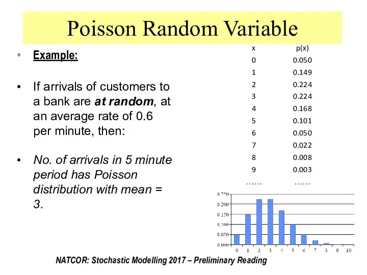
- 23. Example: If arrivals of customers to a bank are at random, at an average rate of
- 24. Continuous Random Variables A random variable is a numerical description of the outcome of an experiment.
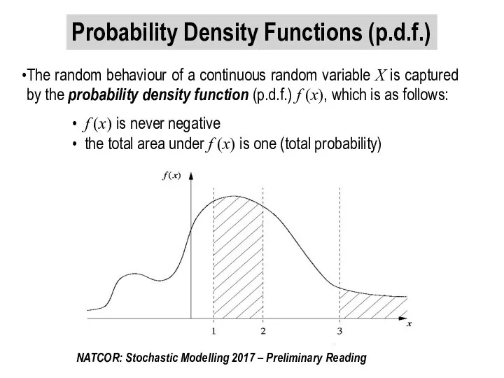
- 25. Probability Density Functions (p.d.f.) The random behaviour of a continuous random variable X is captured by
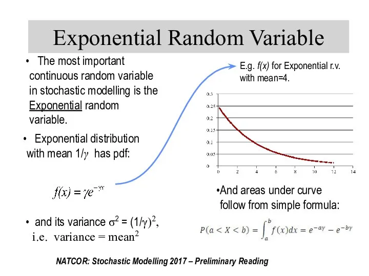
- 26. Probabilities involving X are obtained by determining the area under the pdf, i.e. f (x), for
- 27. Expected value and variance of continuous random variables The expected value, or mean, of a continuous
- 28. Expected value and variance of combinations of continuous random variables NB. Exactly same as for discrete
- 29. Law of Total Probability for Expected Values of a continuous random variable NB. Exactly same as
- 30. Exponential Random Variable The most important continuous random variable in stochastic modelling is the Exponential random
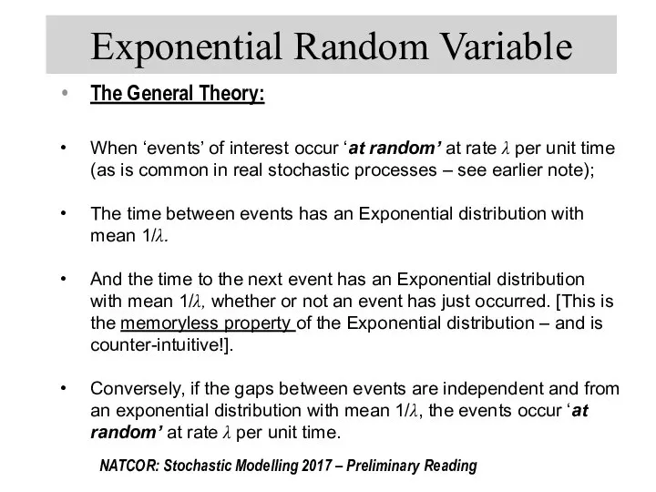
- 31. The General Theory: When ‘events’ of interest occur ‘at random’ at rate λ per unit time
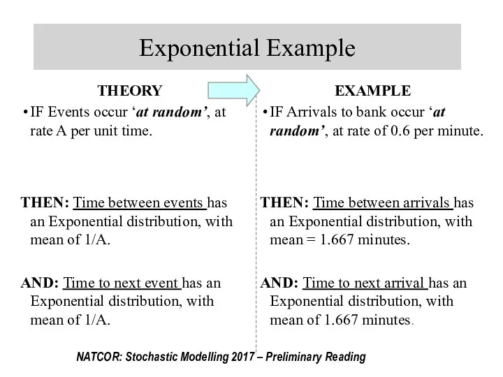
- 32. Exponential Example THEORY IF Events occur ‘at random’, at rate A per unit time. THEN: Time
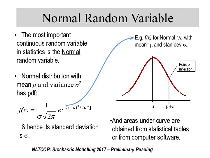
- 33. Normal Random Variable The most important continuous random variable in statistics is the Normal random variable.
- 34. Standardised Normal Random Variable Areas under any Normal curve (mean=μ & SD=σ) can be found by
- 36. Скачать презентацию

Overview
Basic Probability
Discrete Random Variables
Continuous Random Variables
Concepts
Laws and Notation
Conditional Probability
Total Law
Overview
Basic Probability
Discrete Random Variables
Continuous Random Variables
Concepts
Laws and Notation
Conditional Probability
Total Law
BASIC PROBABILITY CONCEPTS: ‘Experiments’ and ‘Events’
Experiment: an action whose outcome
BASIC PROBABILITY CONCEPTS: ‘Experiments’ and ‘Events’
Experiment: an action whose outcome
How to measure probability
Probability: measure of how likely an event is
How to measure probability
Probability: measure of how likely an event is
EX: As part of a survey on whether to ban smoking
EX: As part of a survey on whether to ban smoking
Probability that a person chosen randomly (i.e. everyone has an equal
Probability that a person chosen randomly (i.e. everyone has an equal
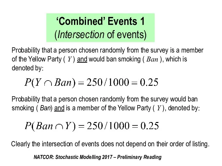
Probability that a person chosen randomly from the survey is a
Probability that a person chosen randomly from the survey is a
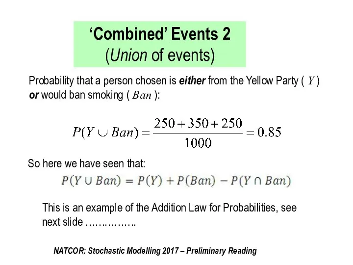
Probability that a person chosen is either from the Yellow Party
Probability that a person chosen is either from the Yellow Party
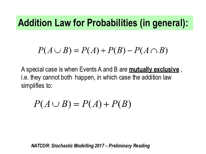
Addition Law for Probabilities (in general):
A special case is when Events
Addition Law for Probabilities (in general):
A special case is when Events

The Conditional Probability that a randomly chosen person would ban smoking
The Conditional Probability that a randomly chosen person would ban smoking
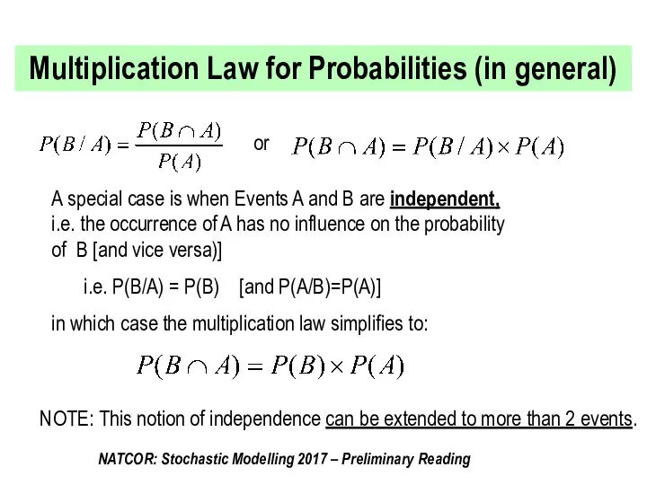
Multiplication Law for Probabilities (in general)
or
A special case is when Events
Multiplication Law for Probabilities (in general)
or
A special case is when Events
Law of Total Probability
EX: The results of the survey on whether
Law of Total Probability
EX: The results of the survey on whether
Law of Total Probability in general
Suppose events A1, A2, A3, …
Law of Total Probability in general
Suppose events A1, A2, A3, …
Tree Diagrams also help think about probabilities
In a factory, a brand
Tree Diagrams also help think about probabilities
In a factory, a brand
Discrete Random Variables
A random variable is a numerical description of the
Discrete Random Variables
A random variable is a numerical description of the

Probability Mass Function (pmf)
of a discrete random variable
The pmf, p(x), of
Probability Mass Function (pmf)
of a discrete random variable
The pmf, p(x), of
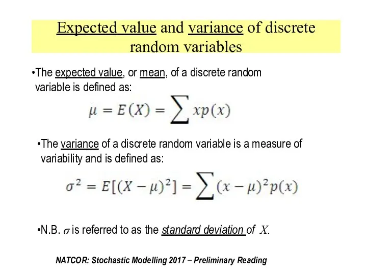
Expected value and variance of discrete random variables
The expected value, or
Expected value and variance of discrete random variables
The expected value, or
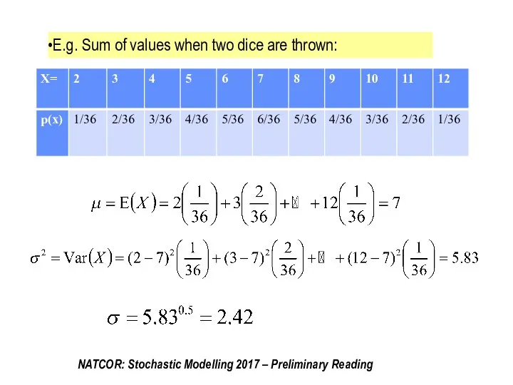
E.g. Sum of values when two dice are thrown:
E.g. Sum of values when two dice are thrown:
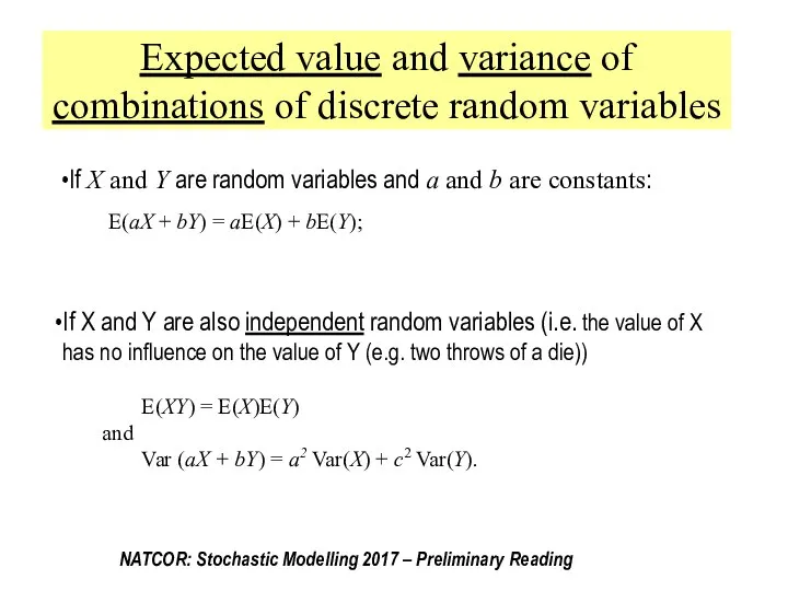
Expected value and variance of combinations of discrete random variables
If X
Expected value and variance of combinations of discrete random variables
If X
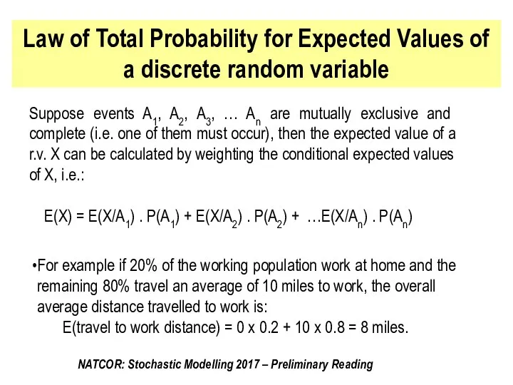
Law of Total Probability for Expected Values of a discrete random
Law of Total Probability for Expected Values of a discrete random
Poisson Random Variable
The most important discrete random variable in stochastic
Poisson Random Variable
The most important discrete random variable in stochastic

The General Theory:
When ‘events’ of interest occur ‘at random’ at rate
The General Theory:
When ‘events’ of interest occur ‘at random’ at rate
Example:
If arrivals of customers to a bank are at random, at
Example:
If arrivals of customers to a bank are at random, at
Continuous Random Variables
A random variable is a numerical description of the
Continuous Random Variables
A random variable is a numerical description of the
Probability Density Functions (p.d.f.)
The random behaviour of a continuous random variable
Probability Density Functions (p.d.f.)
The random behaviour of a continuous random variable
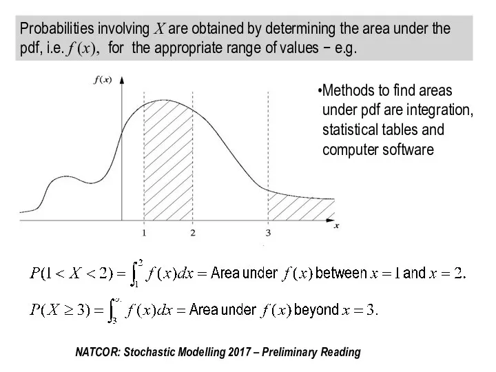
Probabilities involving X are obtained by determining the area under the
Probabilities involving X are obtained by determining the area under the
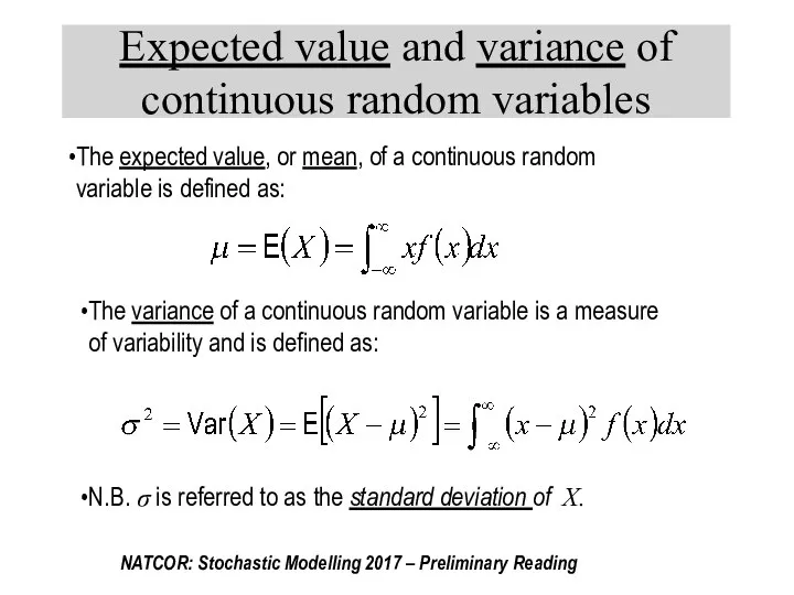
Expected value and variance of continuous random variables
The expected value, or
Expected value and variance of continuous random variables
The expected value, or
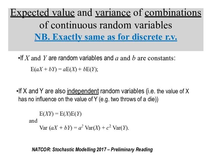
Expected value and variance of combinations of continuous random variables
NB. Exactly
Expected value and variance of combinations of continuous random variables NB. Exactly
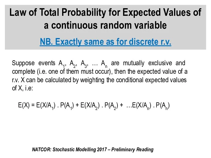
Law of Total Probability for Expected Values of a continuous random
Law of Total Probability for Expected Values of a continuous random
Exponential Random Variable
The most important continuous random variable in stochastic
Exponential Random Variable
The most important continuous random variable in stochastic
The General Theory:
When ‘events’ of interest occur ‘at random’ at rate
The General Theory:
When ‘events’ of interest occur ‘at random’ at rate
Exponential Example
THEORY
IF Events occur ‘at random’, at rate A per unit
Exponential Example
THEORY
IF Events occur ‘at random’, at rate A per unit
Normal Random Variable
The most important continuous random variable in statistics
Normal Random Variable
The most important continuous random variable in statistics
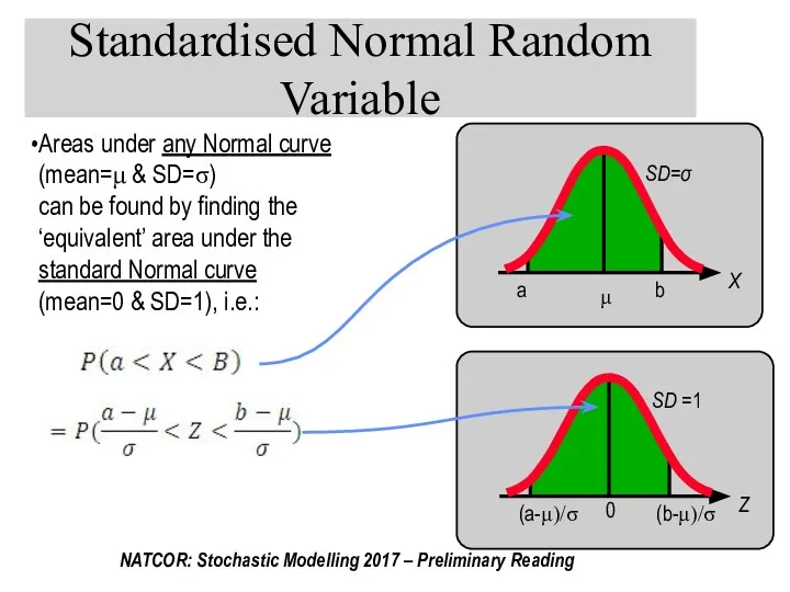
Standardised Normal Random Variable
Areas under any Normal curve (mean=μ & SD=σ)
Standardised Normal Random Variable
Areas under any Normal curve (mean=μ & SD=σ)
 Скрещивающиеся прямые
 Исследование систем уравнений, содержащих параметр.
 Треугольник. Элементы треугольника
 Вейвлет-преобразование изображений
 Лекция 1. Дифференциальное исчисление функции одной переменной
 Векторы в пространстве
 Показательная функция, уравнения, неравенства
 Двугранный угол. Задания для устного счета. Упражнение 8
 Отбор корней тригонометрического уравнения с помощью окружности
 Теорема синусов
 Случаи сложения вида +5, +6
 Алгебра. Исторический очерк
 Упрощение выражений. Решение уравнений
 Параллельность прямых
 Параллелограмм. (8 класс)
 Решение простейших тригонометрических уравнений
 Параллелепипед. Куб
 Множества. Операции над множествами
 МАТЕМАТИКА
  Презентация по математике "Числа от 1 до 100" - скачать бесплатно
 Преобразование графиков функций
 Бізді қоршаған әлемдегі үшбұрыштар
 Обыкновенные дроби. Правила сравнения дробей
 Линейная функция. Прямая пропорциональность, взаимное расположение графиков функций. 7 класс
 Координаты на плоскости. 6 класс
 Различные способы решения тригонометрических неравенств
 Степень с натуральным показателем. Задания
 Математическая викторина. 5 – 6 классы