- Probability theory. Probability Distributions Statistical Entropy

Содержание
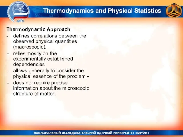
- 2. Thermodynamics and Physical Statistics Thermodynamic Approach - defines correlations between the observed physical quantities (macroscopic), relies
- 3. Statistical Approach - Based on certain models of the micro-structure of matter defines correlations between the
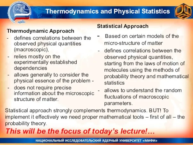
- 4. Thermodynamics and Physical Statistics Statistical approach strongly complements thermodynamics. BUT! To implement it effectively we need
- 5. Probability = the quantitative measure of possibility for certain event to occur. EXAMPLE 1. Eagle and
- 6. Probability = he quantitative measure of possibility for certain event to occur. EXAMPLE 2. Dice game.
- 7. EXAMPLE 3. Rotating of a top toy. If initially the red mark was exactly to the
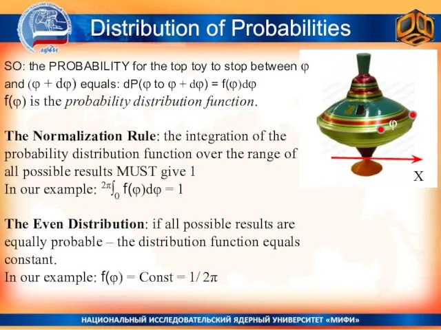
- 8. Distribution of Probabilities X φ SO: the PROBABILITY for the top toy to stop between φ
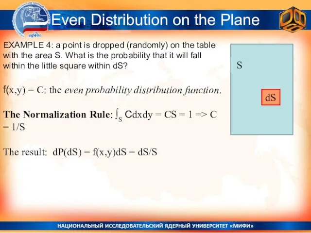
- 9. Even Distribution on the Plane EXAMPLE 4: a point is dropped (randomly) on the table with
- 10. Even Distribution in Physics EXAMPLE 5: Molecules in gas – at the state of thermal equilibrium,
- 11. THE PROPERTIES OF AVERAGES. Average of the sum of two values equals to the sum of
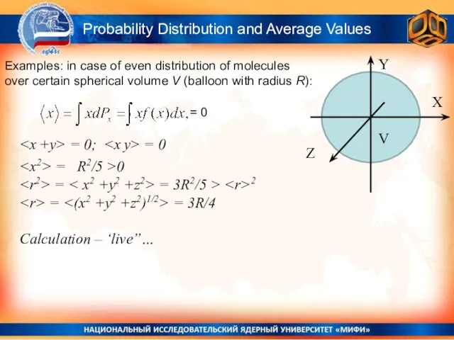
- 12. Probability Distribution and Average Values Examples: in case of even distribution of molecules over certain spherical
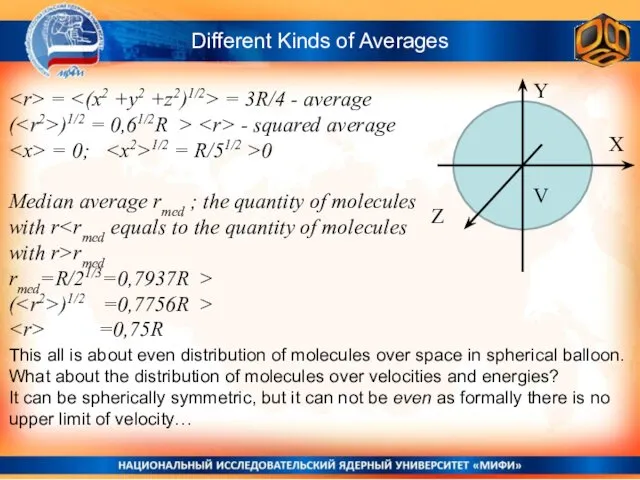
- 13. Different Kinds of Averages Y X Z V = = 3R/4 - average ( )1/2 =
- 14. Eagle and Tails game Normal Distribution
- 15. Eagles and Tails Game EXAMPLE 1: One throw of a coin = one Test (N =
- 16. EXAMPLE 2: 1 Test (or one series of tests) = 2 throws of a coin (N
- 17. The product of probabilities: The first test – the probability of result “1” - P1 The
- 18. General Case: The test length = N (N throws = 1 test) All the types of
- 19. The test series has the length N (N throws = attempts) Number of variants to obtain
- 20. BAR CHART Smooth CHART – distribution function x x+a ΔP x SOME MATHEMATICS: the probability distribution
- 21. N – number pf tests, Ni – number of results of the type i Рi –
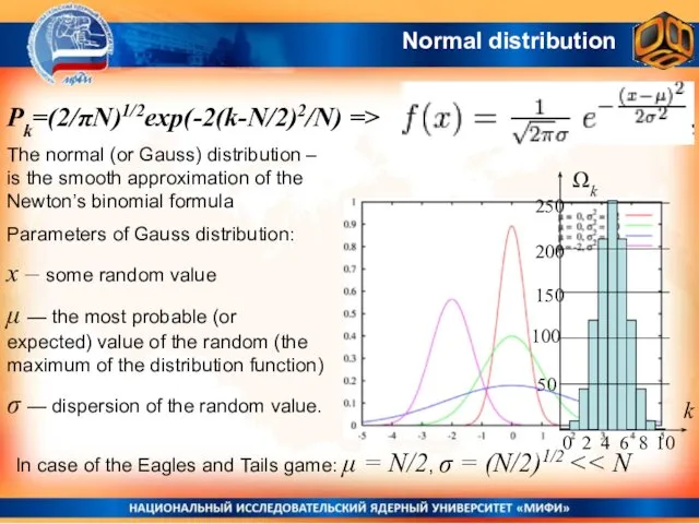
- 22. Normal distribution The normal (or Gauss) distribution – is the smooth approximation of the Newton’s binomial
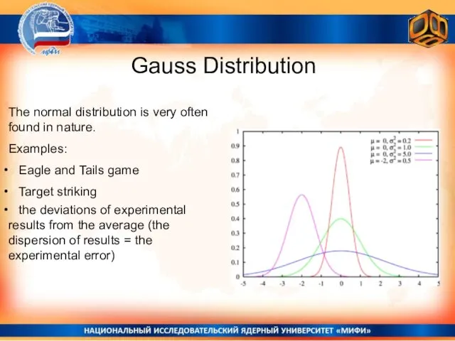
- 23. Gauss Distribution The normal distribution is very often found in nature. Examples: Eagle and Tails game
- 24. Normal (Gauss) Distribution and Entropy MEPhI General Physics
- 25. Number of variants leasing to the result k (if N =10): Ωk= N!/k!(N-k)! Normal Distribution. EXAMPLE:
- 26. The Entropy of Probability The definition of the entropy of probability: S(k) = ln(Ωk) - N
- 27. Entropy in Informatics Type of result Realizations k = 0 0000000000 k = 1 1000000000 0100000000
- 28. Entropy in Informatics Any information or communication can be coded as a string of zeroes and
- 29. The deffinition of entropy as the measure of disorder (or the measure of informational value) in
- 30. Statistical Entropy in Physics MEPhI General Physics
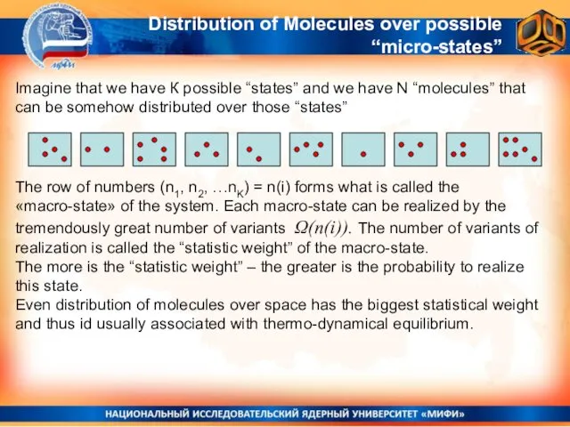
- 31. Distribution of Molecules over possible “micro-states” Imagine that we have К possible “states” and we have
- 32. Statistical Entropy in Molecular Physics: the logarithm of the number of possible micro-realizations of a state
- 33. Entropy is the additive quantity. J/К Statistical Entropy in Physics. For the state of the molecular
- 34. Not a strict proof, but plausible considerations. ~ Statistical Entropy and the Entropy of Ideal Gas
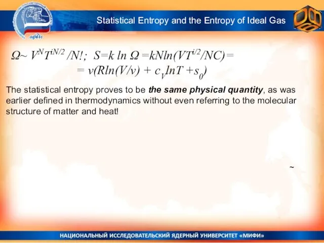
- 35. ~ Statistical Entropy and the Entropy of Ideal Gas Ω~ VNTiN/2 /N!; S=k ln Ω =kNln(VTi/2/NC)=
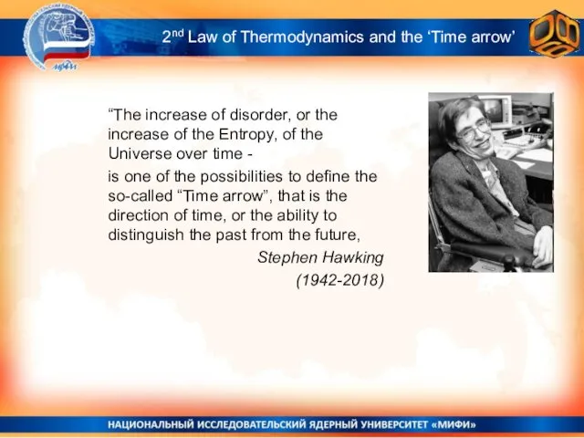
- 36. 2nd Law of Thermodynamics and the ‘Time arrow’ “The increase of disorder, or the increase of
- 37. The Distributions of Molecules over Velocities and Energies Maxwell and Boltzmann Distributions That will be the
- 39. Скачать презентацию
Thermodynamics and Physical Statistics
Thermodynamic Approach
- defines correlations between the observed physical
Thermodynamics and Physical Statistics
Thermodynamic Approach
- defines correlations between the observed physical
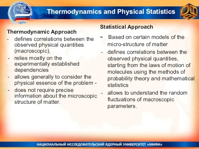
Statistical Approach
- Based on certain models of the micro-structure of matter
defines
Statistical Approach
- Based on certain models of the micro-structure of matter
defines
Thermodynamics and Physical Statistics
Statistical approach strongly complements thermodynamics. BUT! To implement
Thermodynamics and Physical Statistics
Statistical approach strongly complements thermodynamics. BUT! To implement
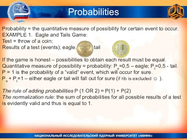
Probability = the quantitative measure of possibility for certain event to
Probability = the quantitative measure of possibility for certain event to
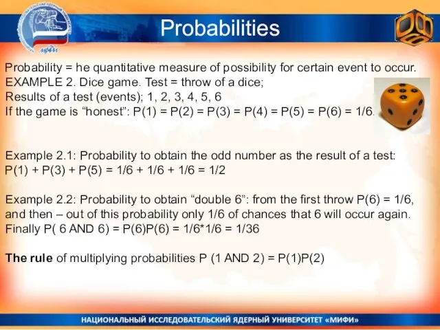
Probability = he quantitative measure of possibility for certain event to
Probability = he quantitative measure of possibility for certain event to
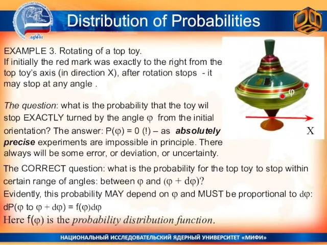
EXAMPLE 3. Rotating of a top toy.
If initially the red
EXAMPLE 3. Rotating of a top toy.
If initially the red
Distribution of Probabilities
X
φ
SO: the PROBABILITY for the top toy to stop
Distribution of Probabilities
X
φ
SO: the PROBABILITY for the top toy to stop
Even Distribution on the Plane
EXAMPLE 4: a point is dropped (randomly)
Even Distribution on the Plane
EXAMPLE 4: a point is dropped (randomly)
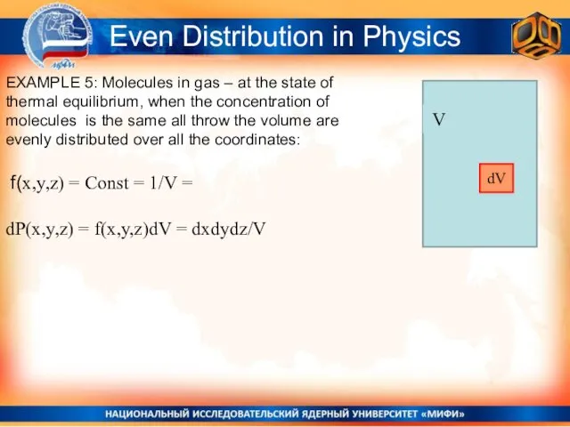
Even Distribution in Physics
EXAMPLE 5: Molecules in gas – at the
Even Distribution in Physics
EXAMPLE 5: Molecules in gas – at the
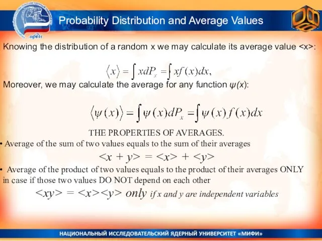
THE PROPERTIES OF AVERAGES.
Average of the sum of two values
THE PROPERTIES OF AVERAGES.
Average of the sum of two values
Probability Distribution and Average Values
Examples: in case of even distribution of
Probability Distribution and Average Values
Examples: in case of even distribution of
Different Kinds of Averages
Y
X
Z
V
= <(x2 +y2 +z2)1/2> = 3R/4 -
Different Kinds of Averages
Y
X
Z
V
Eagle and Tails game
Normal Distribution
Normal Distribution
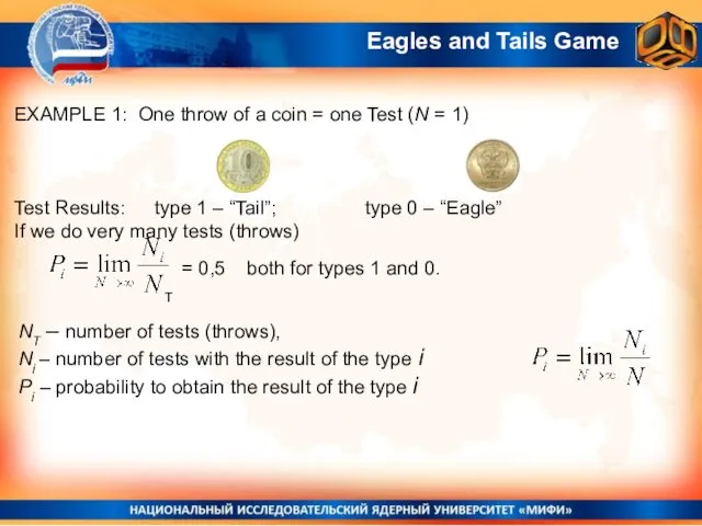
Eagles and Tails Game
EXAMPLE 1: One throw of a coin =
Eagles and Tails Game
EXAMPLE 1: One throw of a coin =
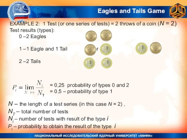
EXAMPLE 2: 1 Test (or one series of tests) = 2
EXAMPLE 2: 1 Test (or one series of tests) = 2
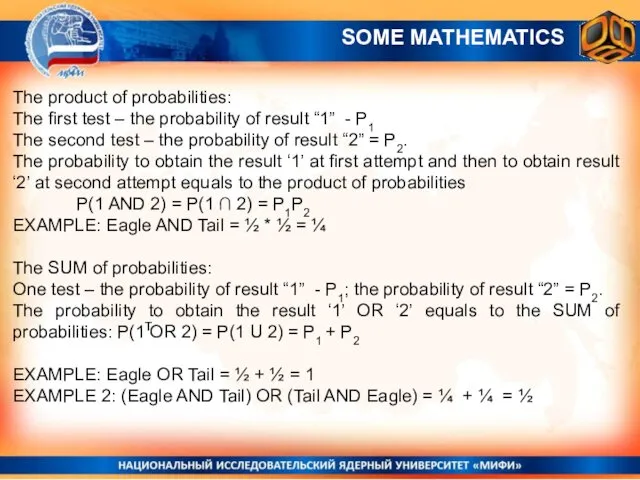
The product of probabilities:
The first test – the probability of
The first test – the probability of
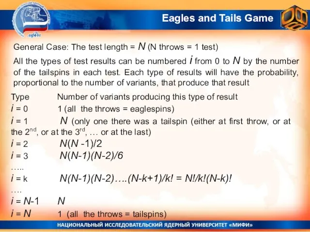
General Case: The test length = N (N throws = 1
General Case: The test length = N (N throws = 1
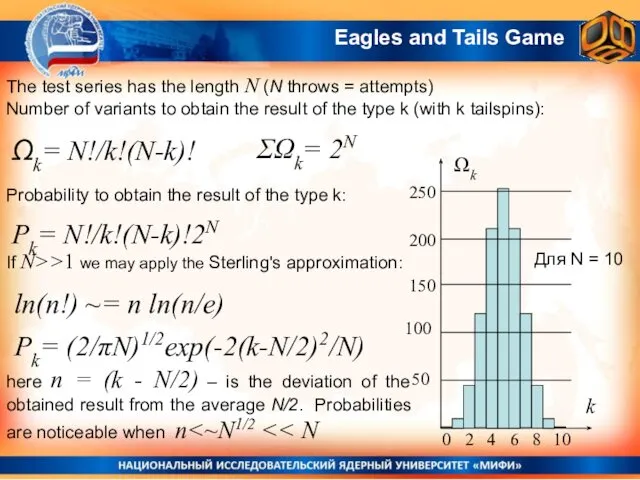
The test series has the length N (N throws = attempts)
Number
The test series has the length N (N throws = attempts)
Number
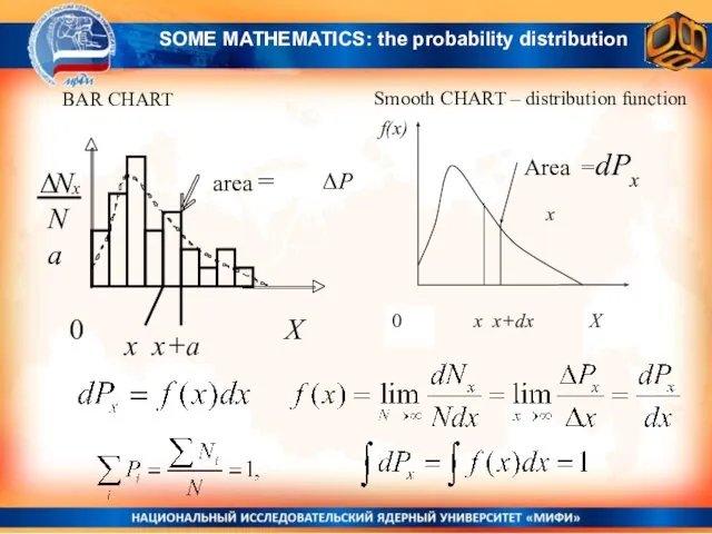
BAR CHART
Smooth CHART – distribution function
x x+a
ΔP
x
SOME MATHEMATICS: the probability
BAR CHART
Smooth CHART – distribution function
x x+a
ΔP
x
SOME MATHEMATICS: the probability
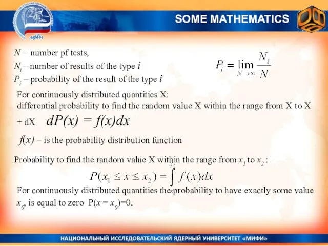
N – number pf tests,
Ni – number of results of
N – number pf tests,
Ni – number of results of
Normal distribution
The normal (or Gauss) distribution – is the smooth approximation
Normal distribution
The normal (or Gauss) distribution – is the smooth approximation
Gauss Distribution
The normal distribution is very often found in nature.
Examples:
Gauss Distribution
The normal distribution is very often found in nature.
Examples:
Normal (Gauss) Distribution
and Entropy
MEPhI General Physics
and Entropy
MEPhI General Physics
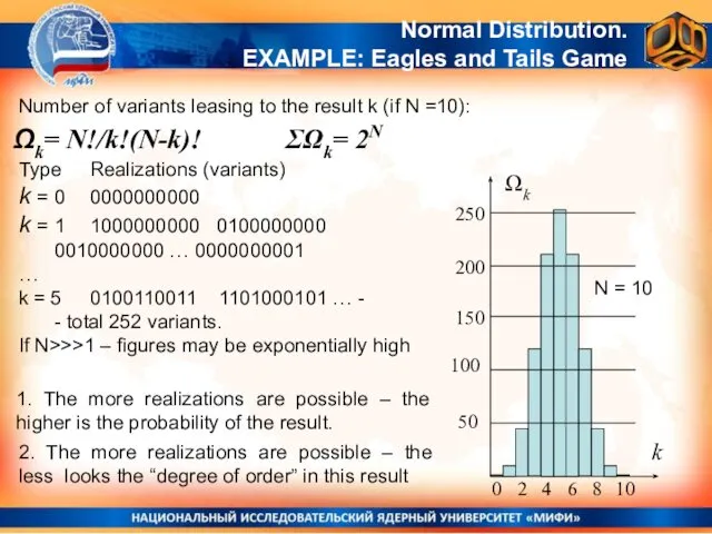
Number of variants leasing to the result k (if N =10):
Ωk=
Number of variants leasing to the result k (if N =10):
Ωk=
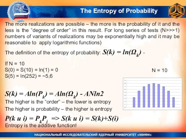
The Entropy of Probability
The definition of the entropy of probability: S(k)
The Entropy of Probability
The definition of the entropy of probability: S(k)
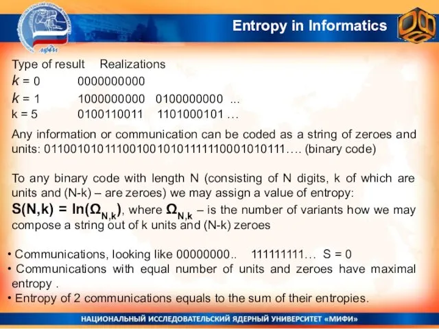
Entropy in Informatics
Type of result Realizations
k = 0 0000000000
k = 1 1000000000 0100000000
Entropy in Informatics
Type of result Realizations
k = 0 0000000000
k = 1 1000000000 0100000000
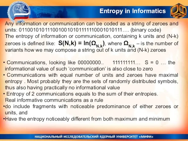
Entropy in Informatics
Any information or communication can be coded as a
Entropy in Informatics
Any information or communication can be coded as a
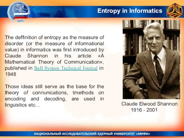
The deffinition of entropy as the measure of disorder (or the
The deffinition of entropy as the measure of disorder (or the
Statistical Entropy in Physics
MEPhI General Physics
MEPhI General Physics
Distribution of Molecules over possible “micro-states”
Imagine that we have К
Distribution of Molecules over possible “micro-states”
Imagine that we have К
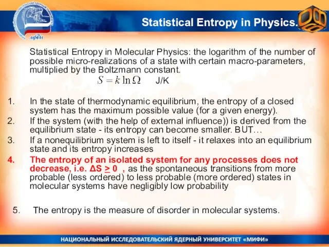
Statistical Entropy in Molecular Physics: the logarithm of the number of
Statistical Entropy in Molecular Physics: the logarithm of the number of
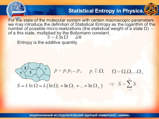
Entropy is the additive quantity.
J/К
Statistical Entropy in Physics.
For
Entropy is the additive quantity.
J/К
Statistical Entropy in Physics.
For
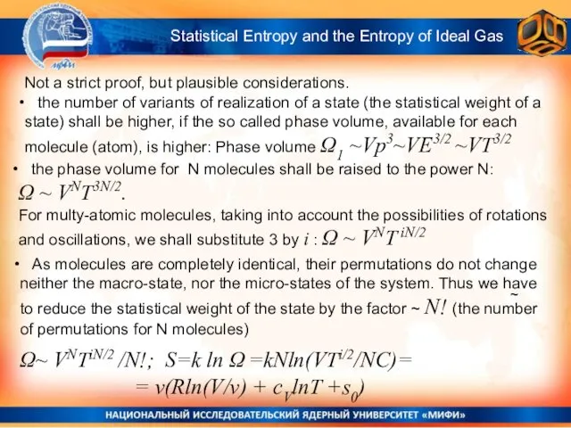
Not a strict proof, but plausible considerations.
~
Statistical Entropy and the
Not a strict proof, but plausible considerations.
~
Statistical Entropy and the
~
Statistical Entropy and the Entropy of Ideal Gas
Ω~ VNTiN/2 /N!; S=k
~
Statistical Entropy and the Entropy of Ideal Gas
Ω~ VNTiN/2 /N!; S=k
2nd Law of Thermodynamics and the ‘Time arrow’
“The increase of disorder,
2nd Law of Thermodynamics and the ‘Time arrow’
“The increase of disorder,
The Distributions of Molecules
over Velocities and Energies
Maxwell and Boltzmann Distributions
That
over Velocities and Energies
Maxwell and Boltzmann Distributions
That
 Решение полного квадратного уравнения
 Теорема Пифагора
 Статистические параметры выборки. Закономерности случайной вариации. Оценка достоверности статистических параметров
 Алгебралық материалдарды оқыту әдістемесі
 Делители и кратные Артамонова Л.В, учитель математики МКОУ «Москаленский лицей»
  Уравнения. урок. 8 класс
 Определение квадратного уравнения. Неполные квадратные уравнения
 Знаходження площі геометричної фігури
 Метод обобщений в статистике. (Лекция 4)
 Системы линейных уравнений и методы их решения. (Тема 2)
 Теория графов. Задача коммивояжера
 Презентация на тему Сравнение предметов Математика 1 класс
 Проверка домашнего задания
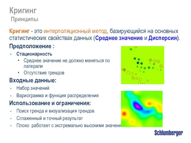 Кригинг
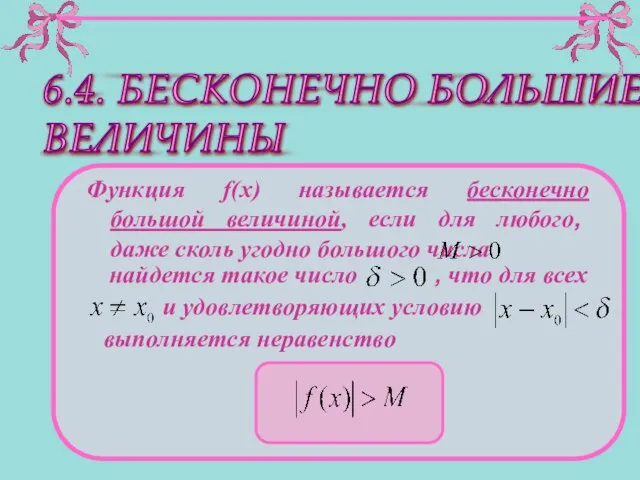 Бесконечно большие величины
 Презентация по математике "Локальные компьютерные сети" - скачать
  Бір айнымалысы бар сызықтық теңдеулерді шешу
 Применение ИКТ на уроках математики, как средство формирования УУД у школьников
 Презентация на тему Неравенства
  Каков развивающий потенциал функциональной линии в курсе математики?
 Урок математики в 6 классе специальной (коррекционной) школы VIII вида по теме «Решение задач в 2-3 действия»
 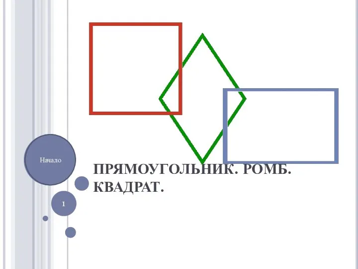 Прямоугольник. Ромб. Квадрат
 Характеристическое свойство арифметической прогрессии
 Построение схемы по данному условию задачи
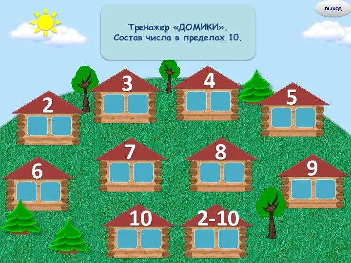 Домики чисел в пределах 10
 Оценка достоверности относительных и средних величин
 Теорема о пропорциональных отрезках. Теорема Фалеса 2
 Определение производной