Quantitative flow cytometry. Advancing the ability of flow cytometry to serve clinical and research purposes
- Quantitative flow cytometry. Advancing the ability of flow cytometry to serve clinical and research purposes

Содержание
- 2. My story : Biysk
- 3. My story : Novosibirsk Biysk
- 4. My story : Novosibirsk B.S. and M.S. in Physics
- 5. My story : Novosibirsk Ph.D. in Physics and Mathematics
- 6. My story : Novosibirsk Ph.D. in Physics and Mathematics Brno Ph.D. in Biophysics
- 7. My story : Novosibirsk Brno Stanford, CA
- 8. What is the problem? Flow cytometry is an essential tool for basic immunological research, clinical discovery
- 9. To develop methods and procedures to enable quantitative measurements of biological substances such as cells, proteins,
- 10. Accurate classification and enumeration of cells with specific phenotypic characteristics. Quantitation of expression levels of surface
- 11. Classification and enumeration of cells with specific phenotypic characteristics Marginal Zone B cells Follicular B cells
- 12. Schematic of the analysis package that statistical procedures are embedded http://cytogenie.org/
- 13. Projection pursuit seeks one projection at a time http://www.few.vu.nl/~tvpham/images/ppde.jpg http://slideplayer.com/slide/4970323/# Projection Pursuit
- 14. why: Curse of dimensionality Less Robustness Required number of events increases with dimensionality Greater computational cost
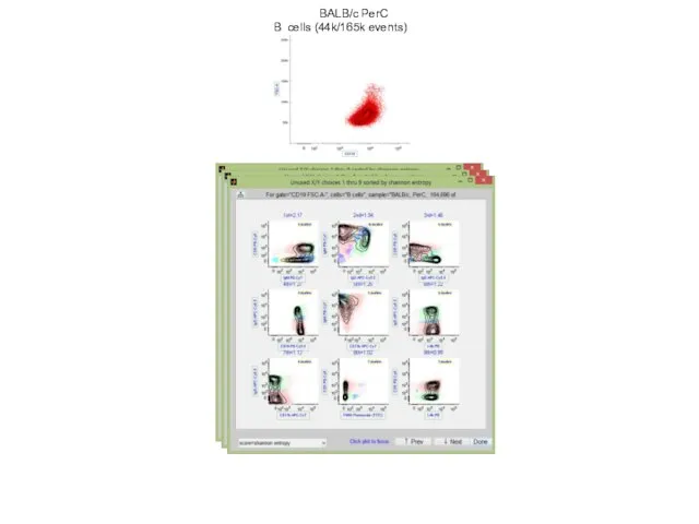
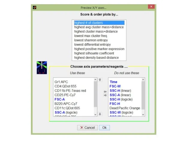
- 15. User-Guided Projection Pursuit
- 16. Walther G. et al, Adv Bioinformatics, 2009 Finding clusters by density based merging (DBM)
- 18. How different are these two samples?
- 19. The index should: possess the properties of a metric: non-negativity d(x,y) ≥ 0 identity of indiscernibles
- 20. Some test statistics are limited to univariate data, e.g., Kolmogorov-Smirnoff statistic and Overton Subtraction (Sheskin, 2000)
- 21. Probability binning plateaus but EMD increases monotonically as one population moves further from the center of
- 22. EMD is the minimum cost of turning one pile of dirt into the other where the
- 23. Assume two distributions represented by signatures, P = {(p1,wp1),…,(pm,wpm)} and Q={(q1,wq1),…,(qn,wqn)} where pi,qi are bin centroids
- 24. Diagnostic tool for distinguishing cystic fibrosis (CF) from allergic bronchopulmonary aspergillosis (ABPA) in CF Surface CD203c
- 25. Multiparameter diagnostic tool in CF and CF-ABPA Compare basophil response to stimulation with the A. fumigatus
- 26. EMD scores based on expression of two independent flow cytometry markers more accurately distinguish allergic (CF-ABPA)
- 27. Cluster matching
- 28. Quantitation of expression levels of surface and intracellular protein biomarkers
- 29. cell cell cell We previously suggested an antigen concentration quantification approach which utilizes the value of
- 30. Experiment: kinetic of mean fluorescence 0.16 min 1 min 3 min 9 min 27 min Beads
- 31. total number of receptor in the volume unit (free+occupied); mean fluorescence value of cell Mathematical model:
- 32. Obtained distributions of neutrophils on the number (in logarithmic scale) of FcgRIIIb receptors for different donors
- 33. As a solution to this problem we introduce a theoretical approach allowing predicting the binding rate
- 34. Chothia et al., Nature, 1989
- 35. Approximation of antigen binding site shape using rectangular “binding spot” model
- 36. From the binding rate constant k+, it was possible to estimate the radius b of the
- 37. Empirical binding rate constant values and corresponding calculated effective binding site radii for 6 antigen-antibody complexes
- 38. The rate constants estimated using binding site radius value for room temperature are in good agreement
- 39. Physics of chemoreception. HC Berg & EM Purcell, Biophys J 20, 93-219 (1977). Electrical analogue
- 40. Antigen “effective binding site” radius as an equivalent of plate capacitor capacitance “Effective binding site” radius
- 41. Functional epitope
- 42. Comparison of estimates for binding site radius electrostatic analogues with effective binding site radii calculated using
- 43. The rate constants estimated using binding site radius value for room temperature are in good agreement
- 44. Practical application in quantitative agglutination test http://image.slidesharecdn.com/nephlerometryandturbidimetry-150203152442-conversion-gate02/95/nephlerometry-and-turbidimetry-6-638.jpg?cb=1422977133
- 45. Thank you! Darya Orlova, Ph.D. Stanford University School of Medicine Genetics Department Beckman Building, Room B013
- 46. [2] Moskalensky et al., 2015 [3] Xavier et al., 1998 [4] Xavier et al., 1999 I5]
- 47. Number of possible 2-D combinations in n dimensional space:
- 51. Silhouette coefficient
- 52. 1. Calculate silhouette coef. (SC) For each pair of clusters+their noise. Calculate % frequency for each
- 53. Summary of diffusion parameters for six well studied antigen-antibody complexes in water solution
- 55. Скачать презентацию
My story :
Biysk
My story :
Biysk

My story :
Novosibirsk
Biysk
My story :
Novosibirsk
Biysk

My story :
Novosibirsk
B.S. and M.S. in Physics
My story :
Novosibirsk
B.S. and M.S. in Physics

My story :
Novosibirsk
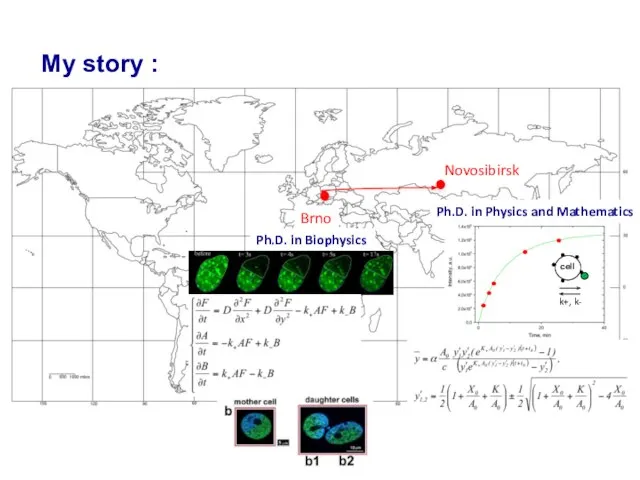
Ph.D. in Physics and Mathematics
My story :
Novosibirsk
Ph.D. in Physics and Mathematics
My story :
Novosibirsk
Ph.D. in Physics and Mathematics
Brno
Ph.D. in Biophysics
My story :
Novosibirsk
Ph.D. in Physics and Mathematics
Brno
Ph.D. in Biophysics
My story :
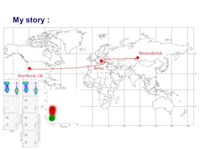
Novosibirsk
Brno
Stanford, CA
My story :
Novosibirsk
Brno
Stanford, CA
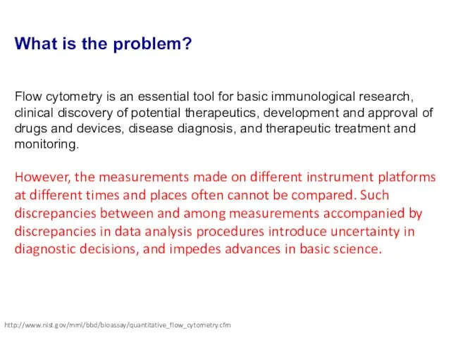
What is the problem?
Flow cytometry is an essential tool for basic
What is the problem?
Flow cytometry is an essential tool for basic

To develop methods and procedures to enable quantitative measurements of biological
To develop methods and procedures to enable quantitative measurements of biological
Accurate classification and enumeration of cells with specific phenotypic characteristics.
Quantitation of
Accurate classification and enumeration of cells with specific phenotypic characteristics.
Quantitation of
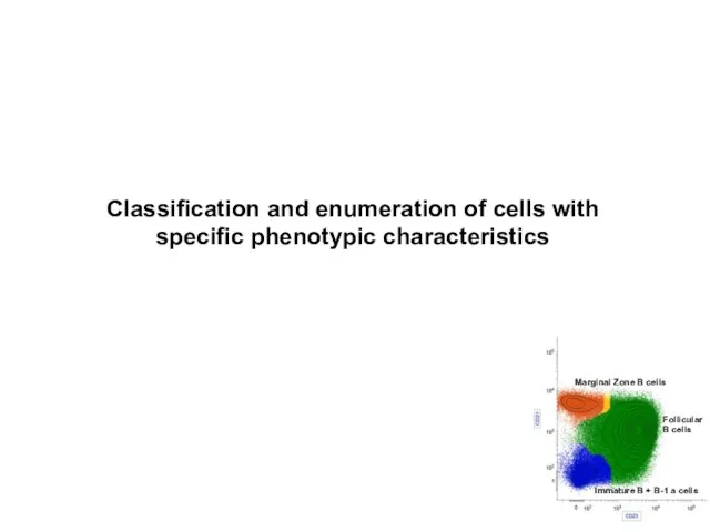
Classification and enumeration of cells with
specific phenotypic characteristics
Marginal Zone
Classification and enumeration of cells with
specific phenotypic characteristics
Marginal Zone

Schematic of the analysis package that statistical procedures are embedded
http://cytogenie.org/
Schematic of the analysis package that statistical procedures are embedded
http://cytogenie.org/

Projection pursuit seeks one projection at a time
http://www.few.vu.nl/~tvpham/images/ppde.jpg
http://slideplayer.com/slide/4970323/#
Projection Pursuit
Projection pursuit seeks one projection at a time
http://www.few.vu.nl/~tvpham/images/ppde.jpg
http://slideplayer.com/slide/4970323/#
Projection Pursuit

why:
Curse of dimensionality
Less Robustness
Required number of events increases with dimensionality
Greater
Curse of dimensionality
Less Robustness
Required number of events increases with dimensionality
Greater
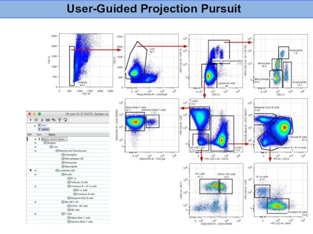
User-Guided Projection Pursuit
User-Guided Projection Pursuit

Walther G. et al, Adv Bioinformatics, 2009
Finding clusters by density based
Walther G. et al, Adv Bioinformatics, 2009
Finding clusters by density based

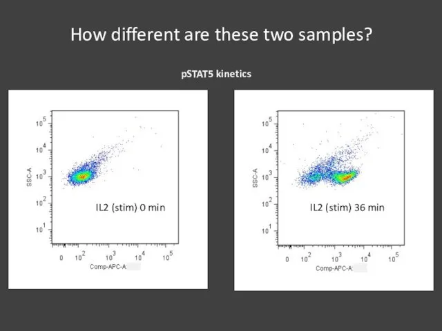
How different are these two samples?
How different are these two samples?

The index should:
possess the properties of a metric:
non-negativity d(x,y) ≥
The index should:
possess the properties of a metric:
non-negativity d(x,y) ≥

Some test statistics are limited to univariate data, e.g., Kolmogorov-Smirnoff statistic
Some test statistics are limited to univariate data, e.g., Kolmogorov-Smirnoff statistic
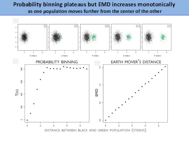
Probability binning plateaus but EMD increases monotonically
as one population moves
Probability binning plateaus but EMD increases monotonically as one population moves

EMD is the minimum cost of turning one pile of dirt
EMD is the minimum cost of turning one pile of dirt
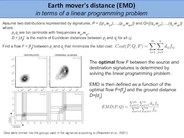
Assume two distributions represented by signatures, P = {(p1,wp1),…,(pm,wpm)} and Q={(q1,wq1),…,(qn,wqn)}
Assume two distributions represented by signatures, P = {(p1,wp1),…,(pm,wpm)} and Q={(q1,wq1),…,(qn,wqn)}

Diagnostic tool for distinguishing cystic fibrosis (CF)
from allergic bronchopulmonary
Diagnostic tool for distinguishing cystic fibrosis (CF) from allergic bronchopulmonary
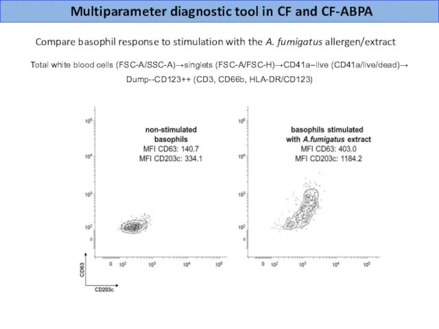
Multiparameter diagnostic tool in CF and CF-ABPA
Compare basophil response to
Multiparameter diagnostic tool in CF and CF-ABPA
Compare basophil response to

EMD scores based on expression of two independent flow cytometry markers
EMD scores based on expression of two independent flow cytometry markers

Cluster matching
Cluster matching

Quantitation of expression levels of surface and intracellular protein biomarkers
Quantitation of expression levels of surface and intracellular protein biomarkers

cell
cell
cell
We previously suggested an antigen concentration quantification approach which utilizes the
cell
cell
cell
We previously suggested an antigen concentration quantification approach which utilizes the

Experiment: kinetic of mean fluorescence
0.16 min
1 min
3 min
9 min
27 min
Beads or
Experiment: kinetic of mean fluorescence
0.16 min
1 min
3 min
9 min
27 min
Beads or

total number of receptor in the volume unit (free+occupied);
mean fluorescence value
total number of receptor in the volume unit (free+occupied);
mean fluorescence value
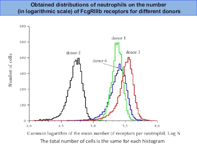
Obtained distributions of neutrophils on the number
(in logarithmic scale) of
Obtained distributions of neutrophils on the number
(in logarithmic scale) of
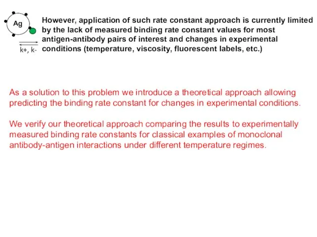
As a solution to this problem we introduce a theoretical approach
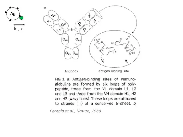
Chothia et al., Nature, 1989
Chothia et al., Nature, 1989

Approximation of antigen binding site shape using rectangular
“binding spot” model
Approximation of antigen binding site shape using rectangular
“binding spot” model

From the binding rate constant k+, it was possible to estimate
From the binding rate constant k+, it was possible to estimate
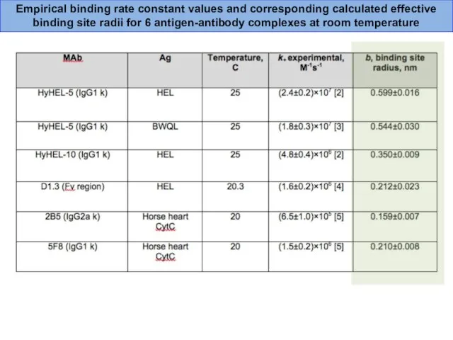
Empirical binding rate constant values and corresponding calculated effective binding site
Empirical binding rate constant values and corresponding calculated effective binding site
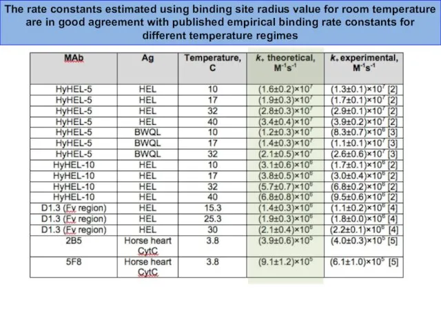
The rate constants estimated using binding site radius value for room
The rate constants estimated using binding site radius value for room
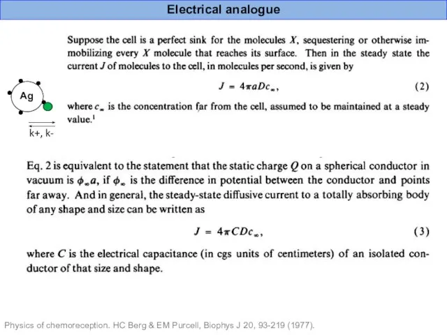
Physics of chemoreception. HC Berg & EM Purcell, Biophys J 20,
Physics of chemoreception. HC Berg & EM Purcell, Biophys J 20,

Antigen “effective binding site” radius as an equivalent of plate capacitor
Antigen “effective binding site” radius as an equivalent of plate capacitor
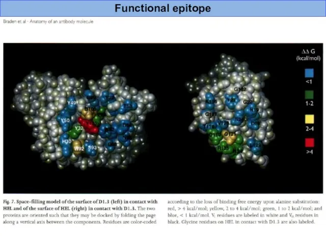
Functional epitope
Functional epitope

Comparison of estimates for binding site radius electrostatic analogues with effective
Comparison of estimates for binding site radius electrostatic analogues with effective
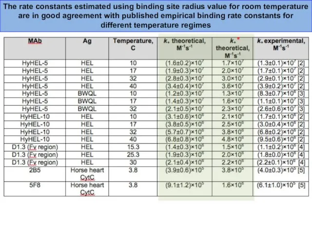
The rate constants estimated using binding site radius value for room
The rate constants estimated using binding site radius value for room
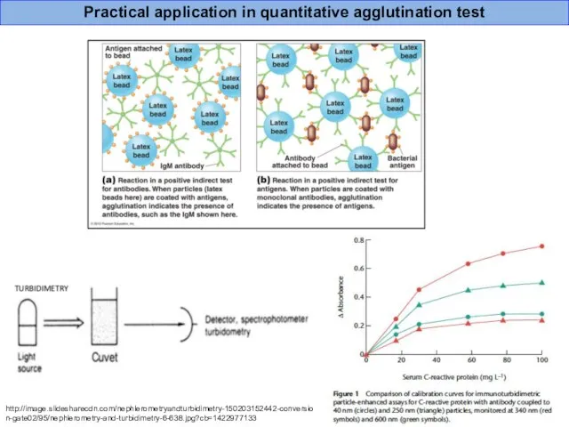
Practical application in quantitative agglutination test
http://image.slidesharecdn.com/nephlerometryandturbidimetry-150203152442-conversion-gate02/95/nephlerometry-and-turbidimetry-6-638.jpg?cb=1422977133
Practical application in quantitative agglutination test
http://image.slidesharecdn.com/nephlerometryandturbidimetry-150203152442-conversion-gate02/95/nephlerometry-and-turbidimetry-6-638.jpg?cb=1422977133

Thank you!
Darya Orlova, Ph.D.
Stanford University School of Medicine
Genetics Department
Beckman Building,
Thank you!
Darya Orlova, Ph.D.
Stanford University School of Medicine
Genetics Department
Beckman Building,
![[2] Moskalensky et al., 2015 [3] Xavier et al., 1998 [4]](/_ipx/f_webp&q_80&fit_contain&s_1440x1080/imagesDir/jpg/510520/slide-45.jpg)
[2] Moskalensky et al., 2015
[3] Xavier et al., 1998
[4] Xavier et
[2] Moskalensky et al., 2015
[3] Xavier et al., 1998
[4] Xavier et

Number of possible 2-D combinations in n dimensional space:
Number of possible 2-D combinations in n dimensional space:

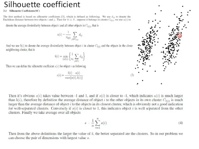
Silhouette coefficient
Silhouette coefficient

1. Calculate silhouette coef. (SC) For each pair of clusters+their noise.
1. Calculate silhouette coef. (SC) For each pair of clusters+their noise.
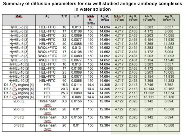
Summary of diffusion parameters for six well studied antigen-antibody complexes
in
Summary of diffusion parameters for six well studied antigen-antibody complexes
in
 Презентация на тему Правила поведения в кабинете биологии и химии.
  Вегетативные органы высших растений. Водоросли
 Физиология слуха и равновесия
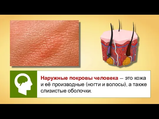 Наружные покровы человек
 Презентация на тему "Моногибридное скрещивание" - скачать презентации по Биологии
 Строение сердца
 Тупорылая Акула
 Презентация на тему Направления эволюции урок в 9 классе
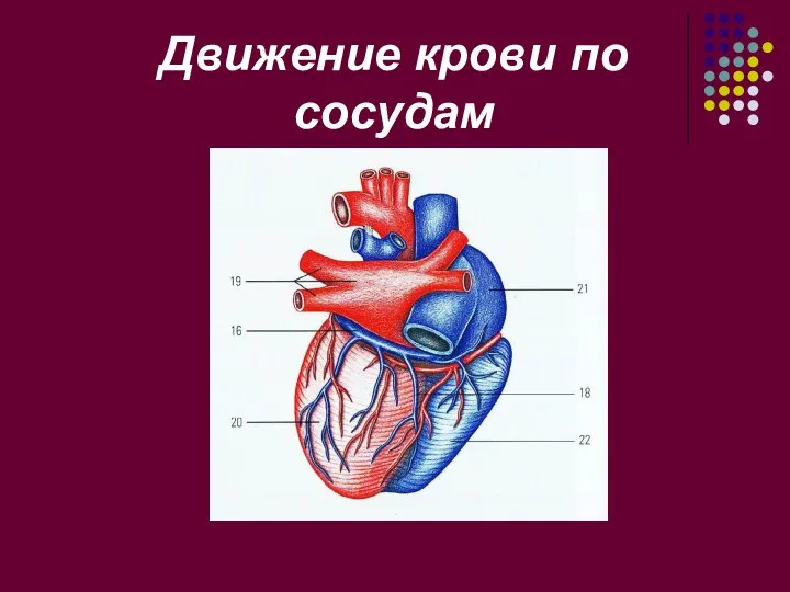 Презентация на тему Движение крови по сосудам
 Российский Государственный Социальный Университет Факультет Охраны труда и Окружающей среды Кафедра социальной экологии П
 Углеводный обмен, фотосинтез, гликолиз
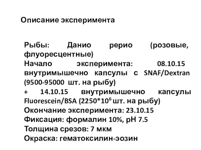 Описание эксперимента. Рыба: Данио рерио
 «Как нерпа приспособилась к жизни в водной среде» Работу выполнила Канахович Александра
 Презентация на тему "Подростковые изменения" - скачать бесплатно презентации по Биологии
 Неклеточные формы жизни: В И Р У С Ы
  Полушария большого мозга
 Будова вуха, слухового та стато-кінетичного аналізаторів
 Тема: «Опорно-двигательная система». Урок 2. Осевой скелет и скелет конечностей. Перечень слайдов: Строение черепа. Строение чер
 Птицы тундры. Выполнила: Серых Виктория, 6 класс МКОУ Пензинская ООШ Новосибирская область Барабинский район Руководитель: Серы
 Нейропсихология внимания
 Нарушения в работе нервной системы и их предупреждение
 Еж. Разновидности ежей. Среда обитания
 Гаметогенез, оплодотворение
 Птицы. Многообразие птичьего мира
 Рефлекс. Рефлекторная дуга
 Презентация по биологии Взаимодействие аллельных и неаллельных генов.
  Класс Птицы
 Гистология. Введение в учение о тканях <number>