- Panel.Methods

Содержание
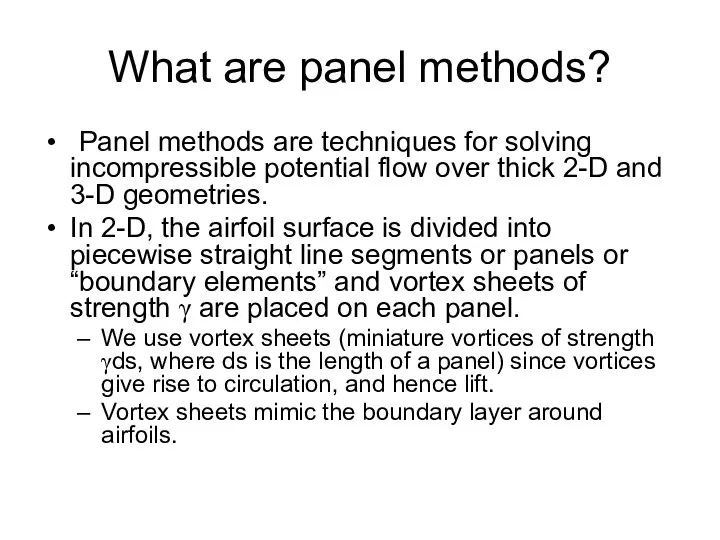
- 2. What are panel methods? Panel methods are techniques for solving incompressible potential flow over thick 2-D
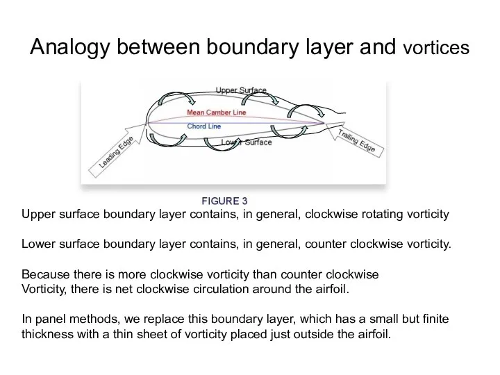
- 3. Analogy between boundary layer and vortices Upper surface boundary layer contains, in general, clockwise rotating vorticity
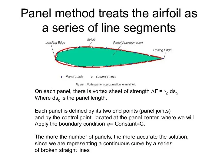
- 4. Panel method treats the airfoil as a series of line segments On each panel, there is
- 5. Boundary Condition We treat the airfoil surface as a streamline. This ensures that the velocity is
- 6. Stream Function due to freestream The free stream is given by Recall This solution satisfies conservation
- 7. Stream function due to a Counterclockwise Vortex of Strengh Γ
- 8. Stream function Vortex, continued.. Pay attention to the signs. A counter-clockwise vortex is considered “positive” In
- 9. Superposition of All Vortices on all Panels In the panel method we use here, ds0 is
- 10. Adding the freestream and vortex effects.. The unknowns are the vortex strength γ0 on each panel,
- 11. Physical meaning of γ0 Panel of length ds0 on the airfoil Its circulation = ΔΓ =
- 12. Pressure distribution and Loads Since V = -γ0
- 13. Kutta Condition Kutta condition states that the pressure above and below the airfoil trailing edge must
- 14. Summing up.. We need to solve the integral equation derived earlier And, satisfy Kutta condition.
- 15. Numerical Procedure We divide the airfoil into N panels. A typical panel is given the number
- 16. Numerical procedure, continued Notice that we use two indices ‘i’ and ‘j’. The index ‘I’ refers
- 17. Numerical procedure, continued.. We thus have N+1 equations for the unknowns γ0,j (j=1…N) and C. We
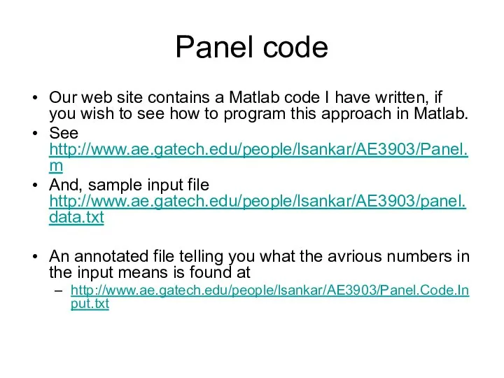
- 18. Panel code Our web site contains a Matlab code I have written, if you wish to
- 20. Скачать презентацию
What are panel methods?
Panel methods are techniques for solving incompressible potential
What are panel methods?
Panel methods are techniques for solving incompressible potential
Analogy between boundary layer and vortices
Upper surface boundary layer contains, in
Analogy between boundary layer and vortices
Upper surface boundary layer contains, in
Panel method treats the airfoil as
a series of line segments
On each
Panel method treats the airfoil as
a series of line segments
On each
Boundary Condition
We treat the airfoil surface as a streamline.
This ensures that
Boundary Condition
We treat the airfoil surface as a streamline.
This ensures that
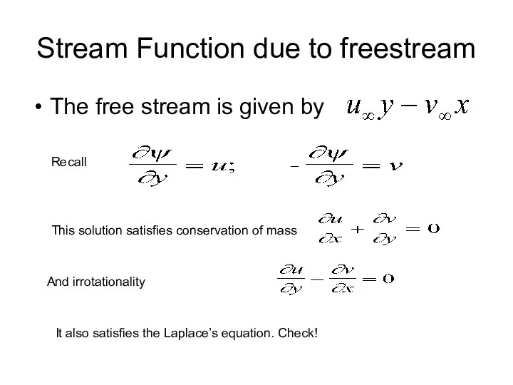
Stream Function due to freestream
The free stream is given by
Recall
Stream Function due to freestream
The free stream is given by
Recall
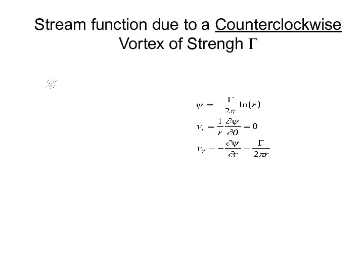
Stream function due to a Counterclockwise Vortex of Strengh Γ
Stream function due to a Counterclockwise Vortex of Strengh Γ
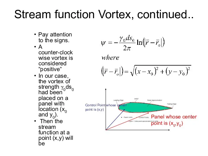
Stream function Vortex, continued..
Pay attention to the signs.
A counter-clockwise vortex is
Stream function Vortex, continued..
Pay attention to the signs.
A counter-clockwise vortex is
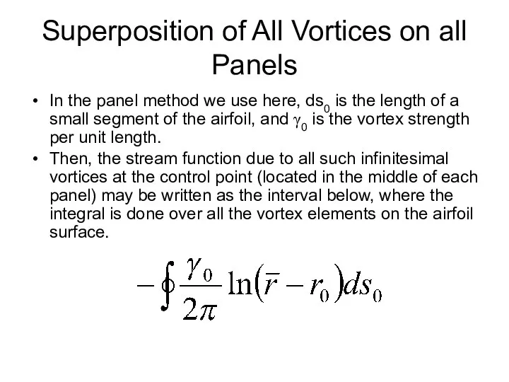
Superposition of All Vortices on all Panels
In the panel method we
Superposition of All Vortices on all Panels
In the panel method we
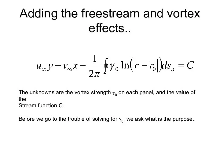
Adding the freestream and vortex effects..
The unknowns are the vortex strength
Adding the freestream and vortex effects..
The unknowns are the vortex strength
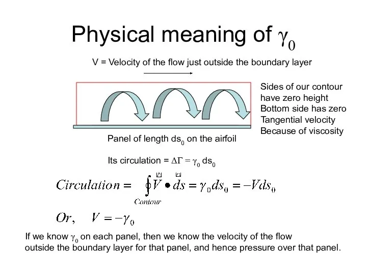
Physical meaning of γ0
Panel of length ds0 on the airfoil
Its circulation
Physical meaning of γ0
Panel of length ds0 on the airfoil
Its circulation
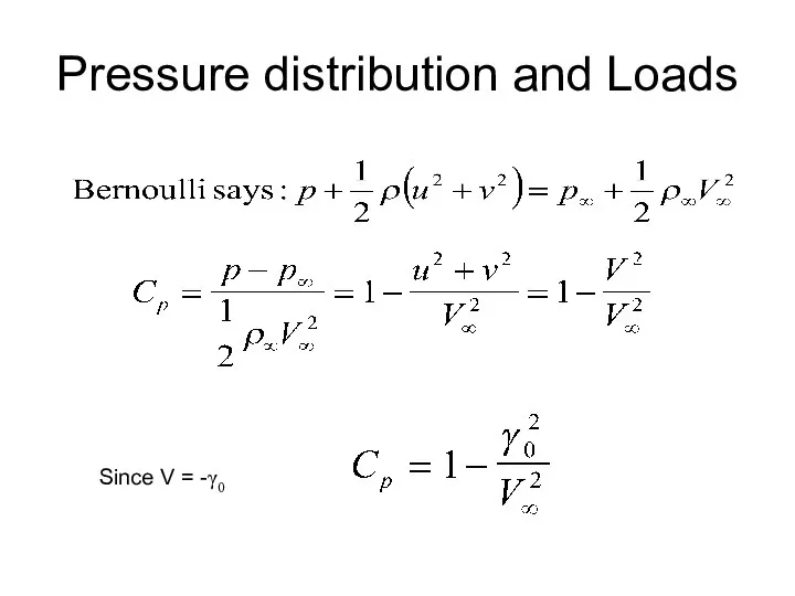
Pressure distribution and Loads
Since V = -γ0
Pressure distribution and Loads
Since V = -γ0
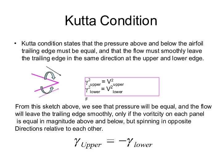
Kutta Condition
Kutta condition states that the pressure above and below the
Kutta Condition
Kutta condition states that the pressure above and below the
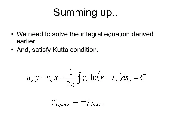
Summing up..
We need to solve the integral equation derived earlier
And, satisfy
Summing up..
We need to solve the integral equation derived earlier
And, satisfy
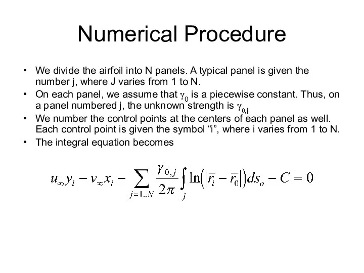
Numerical Procedure
We divide the airfoil into N panels. A typical panel
Numerical Procedure
We divide the airfoil into N panels. A typical panel
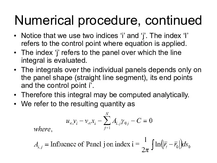
Numerical procedure, continued
Notice that we use two indices ‘i’ and ‘j’.
Numerical procedure, continued
Notice that we use two indices ‘i’ and ‘j’.
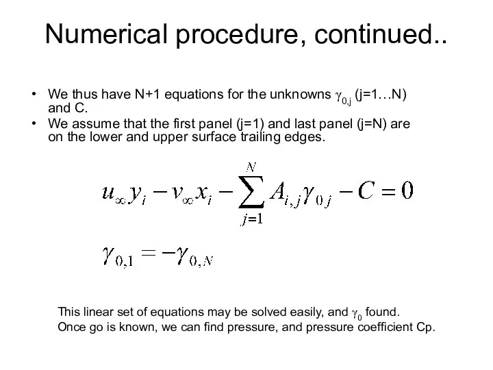
Numerical procedure, continued..
We thus have N+1 equations for the unknowns γ0,j
Numerical procedure, continued..
We thus have N+1 equations for the unknowns γ0,j
Panel code
Our web site contains a Matlab code I have written,
Panel code
Our web site contains a Matlab code I have written,
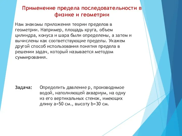 Применение предела последовательности в физике и геометрии
 Тренажёр. Умножение и деление на 5
 Это гордое слово Победа!
 Признаки параллельности двух прямых
 Наибольший общий делитель. Взаимно простые числа
 Презентация на тему Решение задач на смеси, сплавы, растворы
 Составь задачу и реши её с помощью уравнения
 Аттестационная работа. Решение уравнений и задач в целых числах
 Урок математики
 Площадь многоугольников
 Тела вращения
 Признаки делимости
 Семь чудес света: математика 1 класс
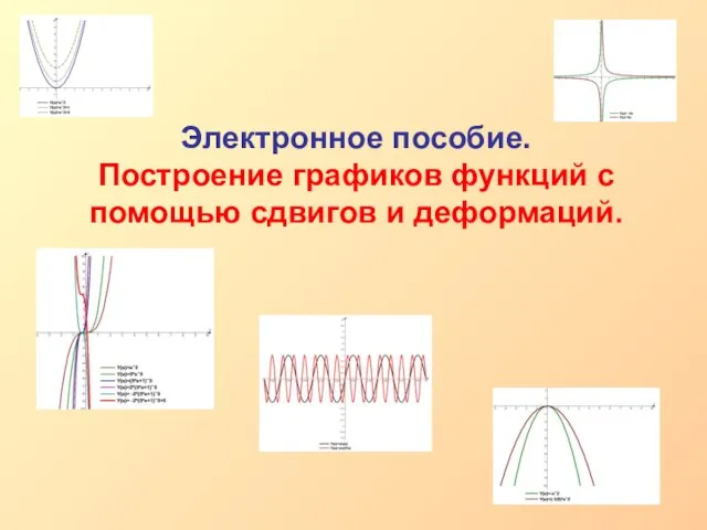 Построение графиков функций с помощью сдвигов и деформаций
 Урок 14. Первый признак равенства треугольников
 Логическая равносильность формул
 Нестандартные задачи как средство формирования исследовательских умений обучающихся в курсе алгебры 8 класс
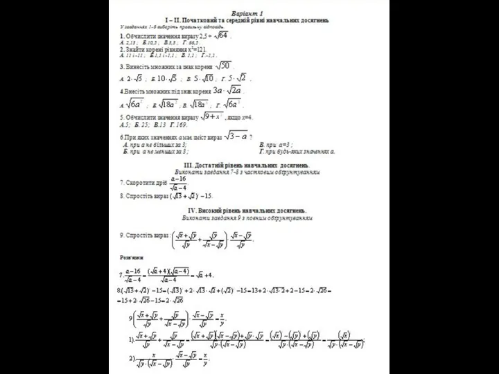 Квадратный корень. Варианты заданий
 Какая цифра в разряде единиц стоит в записи числа 134265?
 Повтарение по математике. Уравнение
 Части графа. Операции над частями графа
 Распределительный закон. История возникновения
 Тела вращения. Цилиндр
 Результаты пробных ЕГЭ по математике (2013-2014 учебный год)
 Решение систем уравнений методом итерации функции. 10 класс
 Контрольная работа по математике
 Метод проектов на уроке математики
 Логические операции И ИЛИ