- Descriptive statistics. Elementary statistics. Larson. Farber. (Chapter 2)

Содержание
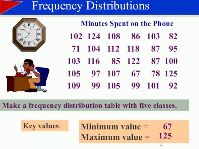
- 2. Frequency Distributions 102 124 108 86 103 82 71 104 112 118 87 95 103 116
- 3. Decide on the number of classes (For this problem use 5) Calculate the Class Width (125
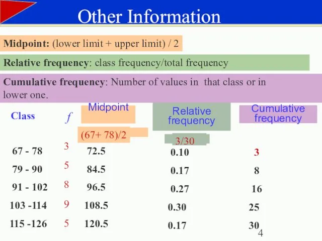
- 4. 67 - 78 79 - 90 91 - 102 103 -114 115 -126 3 5 8
- 5. Boundaries 66.5 - 78.5 78.5 - 90.5 90.5 - 102.5 102.5 -114.5 115.5 -126.5 Frequency Histogram
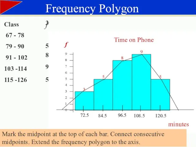
- 6. Frequency Polygon Time on Phone minutes f Mark the midpoint at the top of each bar.
- 7. Relative Frequency Histogram Time on Phone minutes Relative frequency Relative frequency on vertical scale
- 8. Ogive An ogive reports the number of values in the data set that are less than
- 9. Stem-and-Leaf Plot 6 | 7 | 8 | 9 | 10| 11| 12| Stem Leaf Lowest
- 10. Stem-and-Leaf Plot 6 |7 7 |1 8 8 |2 5 6 7 7 9 |2 5
- 11. Stem-and-Leaf with two lines per stem 6 | 7 7 | 1 7 | 8 8
- 12. Dotplot 66 76 86 96 106 116 126 Phone minutes
- 13. The 1995 NASA budget (billions of $) divided among 3 categories. Pie Chart Used to describe
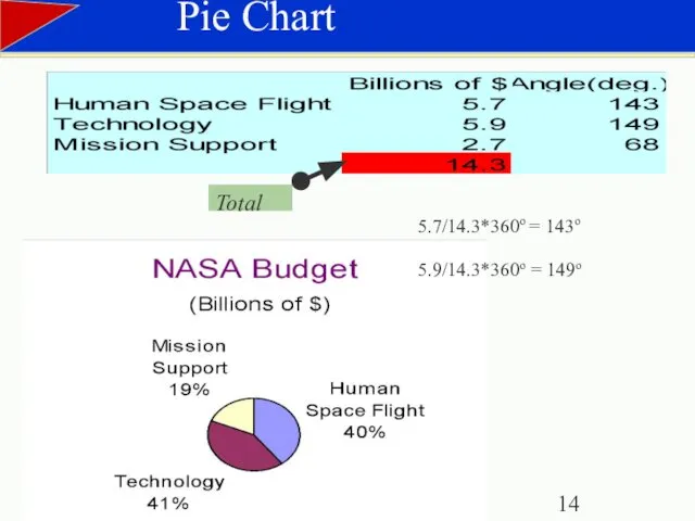
- 14. Pie Chart 5.7/14.3*360o = 143o 5.9/14.3*360o = 149o
- 15. Measures of Central Tendency Mean: The sum of all data values divided by the number of
- 16. 2 4 2 0 40 2 4 3 6 Calculate the mean, the median, and the
- 17. 2 4 2 0 2 4 3 6 Calculate the mean, the median, and the mode
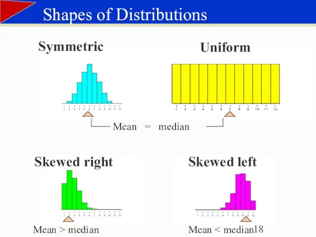
- 18. Shapes of Distributions Uniform Symmetric Skewed right Skewed left Mean > median Mean Mean = median
- 19. Descriptive Statistics Closing prices for two stocks were recorded on ten successive Fridays. Calculate the mean,
- 20. Range for A = 67 - 56 = $11 Range = Maximum value - Minimum value
- 21. -5.5 -5.5 -4.5 -3.5 -0.5 1.5 1.5 5.5 5.5 5.5 56 56 57 58 61 63
- 22. Population Variance: The sum of the squares of the deviations, divided by N. Stock A 56
- 23. Population Standard Deviation Population Standard Deviation The square root of the population variance. The population standard
- 24. Calculate the measures of variation for Stock B Sample Standard Deviation To calculate a sample variance
- 25. Summary Population Standard Deviation Sample Variance Sample Standard Deviation Range = Maximum value - Minimum value
- 26. Empiricl Rule 68- 95- 99.7% rule Data with symmetric bell-shaped distribution has the following characteristics. About
- 27. Using the Empirical Rule The mean value of homes on a street is $125 thousand with
- 28. Chebychev’s Theorem For k = 3, at least 1-1/9 = 8/9= 88.9% of the data lies
- 29. Chebychev’s Theorem The mean time in a women’s 400-meter dash is 52.4 seconds with a standard
- 30. Grouped Data 30 Class f Midpoint (x) To approximate the mean of data in a frequency
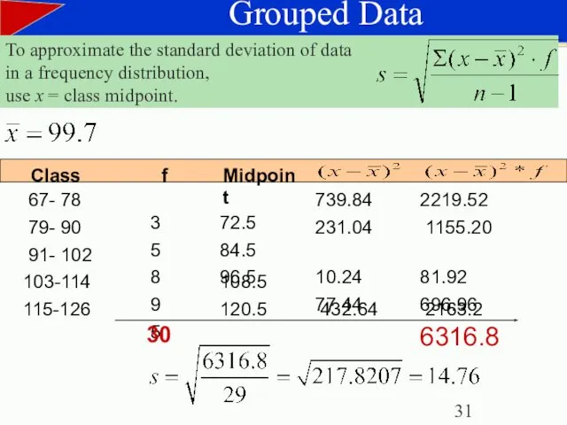
- 31. Grouped Data To approximate the standard deviation of data in a frequency distribution, use x =
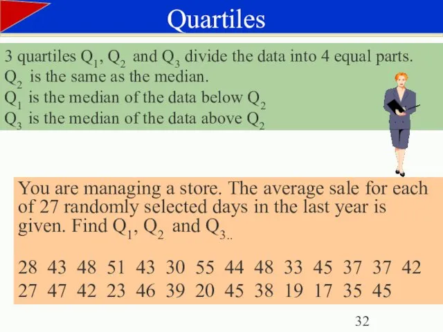
- 32. Quartiles You are managing a store. The average sale for each of 27 randomly selected days
- 33. The data in ranked order (n = 27) are: 17 19 20 23 27 28 30
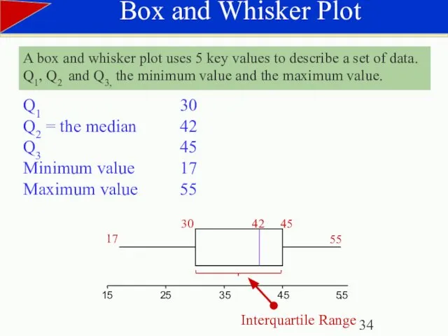
- 34. Box and Whisker Plot A box and whisker plot uses 5 key values to describe a
- 35. Percentiles Percentiles divide the data into 100 parts. There are 99 percentiles: P1, P2, P3…P99 .
- 37. Скачать презентацию
Frequency Distributions
102 124 108 86 103 82
71 104 112 118 87 95
103 116 85 122 87 100
105
Frequency Distributions
102 124 108 86 103 82
71 104 112 118 87 95
103 116 85 122 87 100
105

Decide on the number of classes (For this problem use 5)
Decide on the number of classes (For this problem use 5)
67 - 78
79 - 90
91 - 102
103 -114
115
67 - 78
79 - 90
91 - 102
103 -114
115
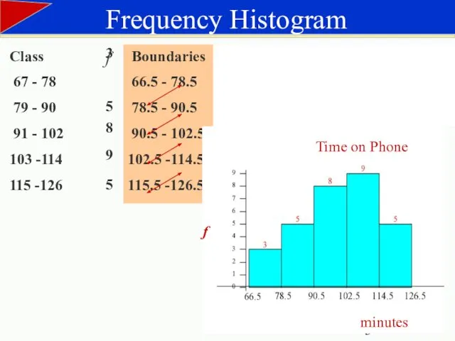
Boundaries
66.5 - 78.5
78.5 - 90.5
90.5 - 102.5
102.5
Boundaries
66.5 - 78.5
78.5 - 90.5
90.5 - 102.5
102.5
Frequency Polygon
Time on Phone
minutes
f
Mark the midpoint at the top of
Frequency Polygon
Time on Phone
minutes
f
Mark the midpoint at the top of
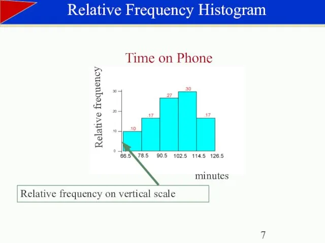
Relative Frequency Histogram
Time on Phone
minutes
Relative frequency
Relative frequency on vertical scale
Relative Frequency Histogram
Time on Phone
minutes
Relative frequency
Relative frequency on vertical scale
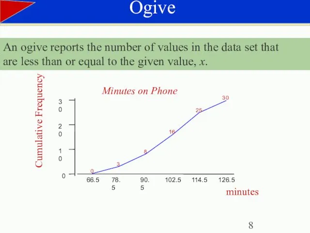
Ogive
An ogive reports the number of values in the data set
Ogive
An ogive reports the number of values in the data set
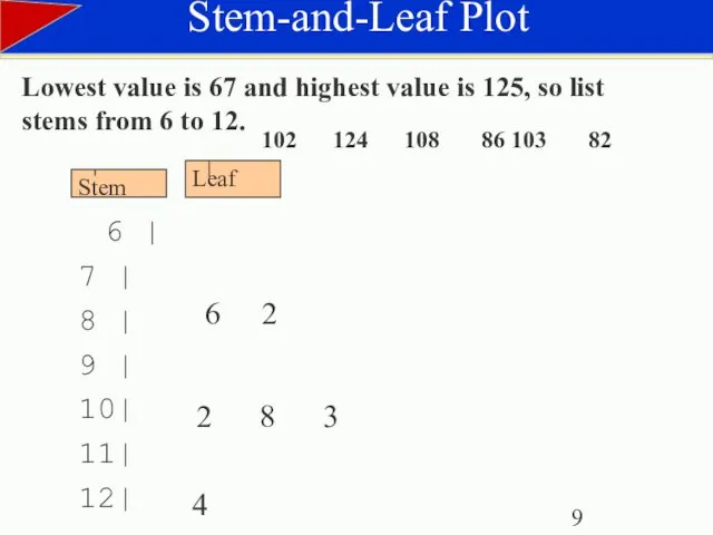
Stem-and-Leaf Plot
6 |
7 |
8 |
9 |
10|
11|
12|
Stem
Leaf
Lowest value is 67
Stem-and-Leaf Plot
6 |
7 |
8 |
9 |
10|
11|
12|
Stem
Leaf
Lowest value is 67
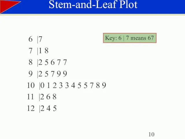
Stem-and-Leaf Plot
6 |7
7 |1 8
8 |2 5 6
Stem-and-Leaf Plot
6 |7
7 |1 8
8 |2 5 6
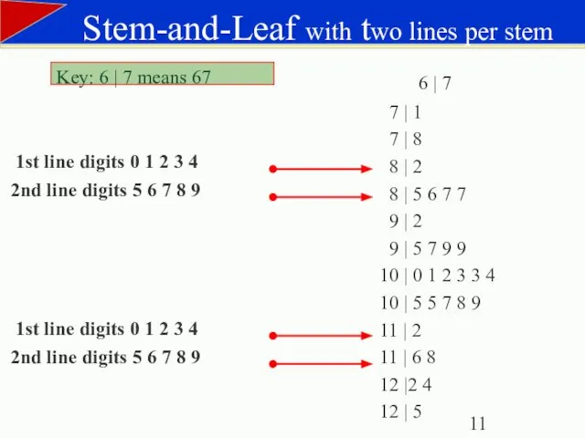
Stem-and-Leaf with two lines per stem
6 | 7
7 |
Stem-and-Leaf with two lines per stem
6 | 7
7 |
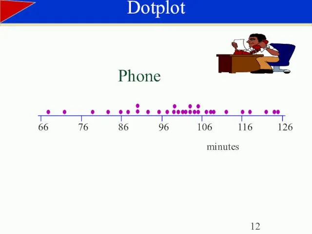
Dotplot
66
76
86
96
106
116
126
Phone
minutes
Dotplot
66
76
86
96
106
116
126
Phone
minutes
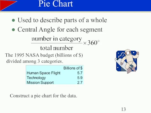
The 1995 NASA budget (billions of $)
divided among 3 categories.
Pie
The 1995 NASA budget (billions of $)
divided among 3 categories.
Pie
Pie Chart
5.7/14.3*360o = 143o
5.9/14.3*360o = 149o
Pie Chart
5.7/14.3*360o = 143o
5.9/14.3*360o = 149o

Measures of Central Tendency
Mean: The sum of all data values divided
Measures of Central Tendency
Mean: The sum of all data values divided
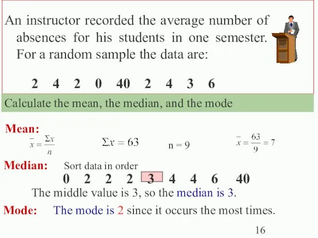
2 4 2 0 40 2 4 3 6
Calculate the mean,
2 4 2 0 40 2 4 3 6
Calculate the mean,
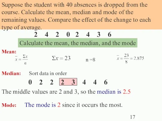
2 4 2 0 2 4 3 6
Calculate the mean, the
2 4 2 0 2 4 3 6
Calculate the mean, the
Shapes of Distributions
Uniform
Symmetric
Skewed right
Skewed left
Mean > median
Mean < median
Mean = median
Shapes of Distributions
Uniform
Symmetric
Skewed right
Skewed left
Mean > median
Mean < median
Mean = median

Descriptive Statistics
Closing prices for two stocks were recorded on ten successive
Descriptive Statistics
Closing prices for two stocks were recorded on ten successive
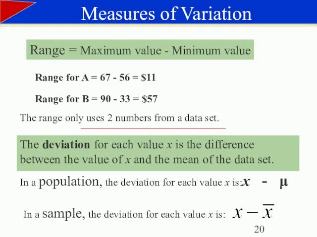
Range for A = 67 - 56 = $11
Range = Maximum
Range for A = 67 - 56 = $11
Range = Maximum
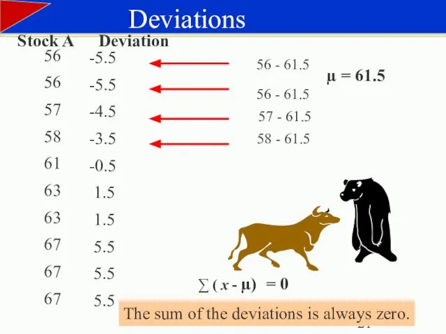
-5.5
-5.5
-4.5
-3.5
-0.5
1.5
-5.5
-5.5
-4.5
-3.5
-0.5
1.5
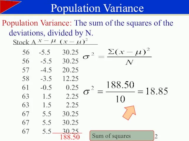
Population Variance: The sum of the squares of the deviations, divided
Population Variance: The sum of the squares of the deviations, divided
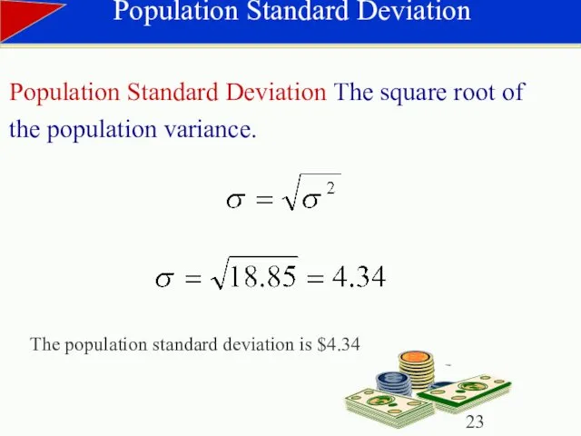
Population Standard Deviation
Population Standard Deviation The square root of the
Population Standard Deviation
Population Standard Deviation The square root of the
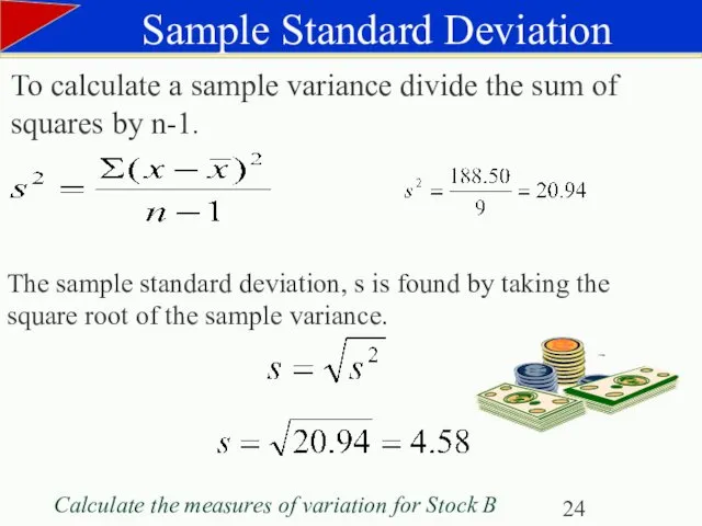
Calculate the measures of variation for Stock B
Sample Standard Deviation
To
Calculate the measures of variation for Stock B
Sample Standard Deviation
To
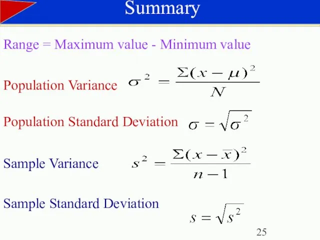
Summary
Population Standard Deviation
Sample Variance
Sample Standard Deviation
Range = Maximum value - Minimum
Summary
Population Standard Deviation
Sample Variance
Sample Standard Deviation
Range = Maximum value - Minimum

Empiricl Rule 68- 95- 99.7% rule
Data with symmetric bell-shaped distribution has
Empiricl Rule 68- 95- 99.7% rule
Data with symmetric bell-shaped distribution has

Using the Empirical Rule
The mean value of homes on a street
Using the Empirical Rule
The mean value of homes on a street
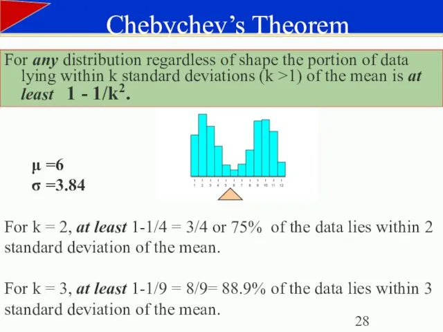
Chebychev’s Theorem
For k = 3, at least 1-1/9 = 8/9= 88.9%
Chebychev’s Theorem
For k = 3, at least 1-1/9 = 8/9= 88.9%
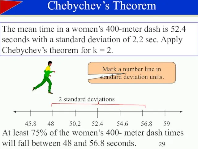
Chebychev’s Theorem
The mean time in a women’s 400-meter dash is 52.4
Chebychev’s Theorem
The mean time in a women’s 400-meter dash is 52.4
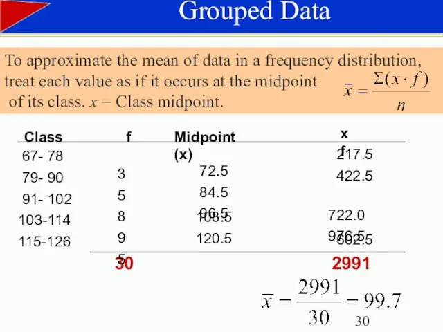
Grouped Data
30
Class
f
Midpoint (x)
To approximate the mean of data in
Grouped Data
30
Class
f
Midpoint (x)
To approximate the mean of data in
Grouped Data
To approximate the standard deviation of data
in a frequency
Grouped Data
To approximate the standard deviation of data
in a frequency
Quartiles
You are managing a store. The average sale for each of
Quartiles
You are managing a store. The average sale for each of
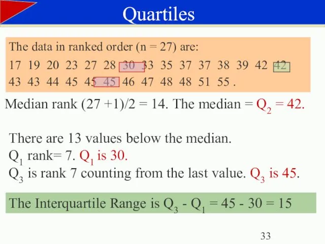
The data in ranked order (n = 27) are:
17 19 20
The data in ranked order (n = 27) are:
17 19 20
Box and Whisker Plot
A box and whisker plot uses 5 key
Box and Whisker Plot
A box and whisker plot uses 5 key
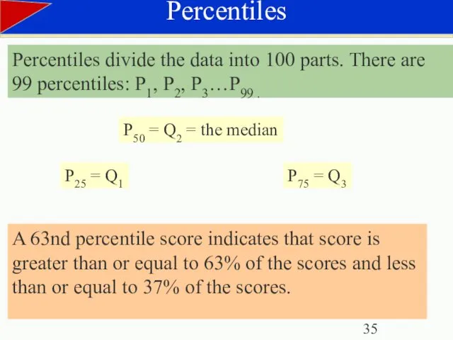
Percentiles
Percentiles divide the data into 100 parts. There are 99 percentiles:
Percentiles
Percentiles divide the data into 100 parts. There are 99 percentiles:
 Использование преобразований тригонометрических выражений при решении заданий ЕГЭ
 Решение тригонометрических уравнений (открытый урок в 10 классе)
 Теорема Пифагора Выполнила Вахтанова Б. С. учитель математики МАОУ СОШ №3 МО г-к Анапа
 Логарифмические уравнения
 Симметрия
 Пропорции (11 класс) - презентация_
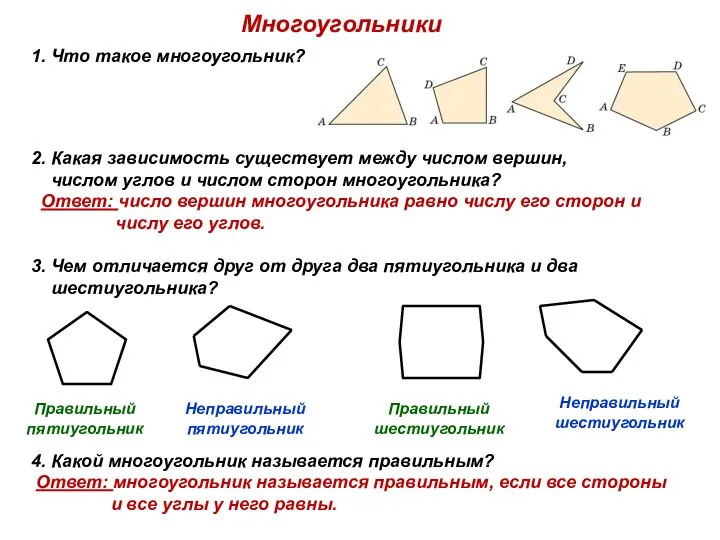 Многоугольники
 Квадратные неравенства. 9 класс
 Число 8. Цифра 8
 Экономические задачи №17
 Матрицы и действия с ними
 Как построена задача, какие части есть в задаче
 Понятие множества. Урок 1. 5 класс
 Математический кружок. Секреты арифметических фокусов
 Объём тел
 Множення раціональних чисел
 Похибки прямих вимірювань
 Формулы сокращенного умножения
 Путешествие в страну Десятичных дробей.
  Деревья. Связность. Дерево и его виды
 Презентация по математике "Число 7" - скачать бесплатно
 Окружность и круг
 Логическое следование
 Числовые выражения
 Математический диктант. 4 класс
 Арифметическая прогрессия
 Трапеция
 Решение задач с помощью дробных рациональных уравнений