- Shortest Paths

Содержание
- 2. The Bellman-Ford algorithm 1958 1962
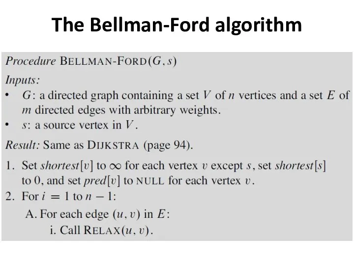
- 3. The Bellman-Ford algorithm
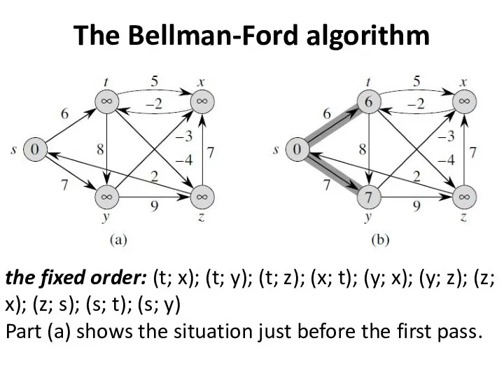
- 4. The Bellman-Ford algorithm the fixed order: (t; x); (t; y); (t; z); (x; t); (y; x);
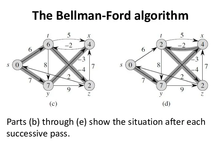
- 5. The Bellman-Ford algorithm Parts (b) through (e) show the situation after each successive pass.
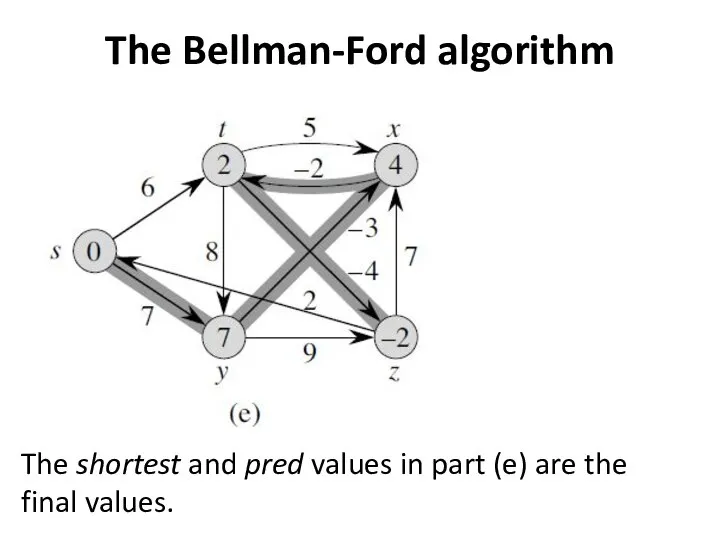
- 6. The Bellman-Ford algorithm The shortest and pred values in part (e) are the final values.
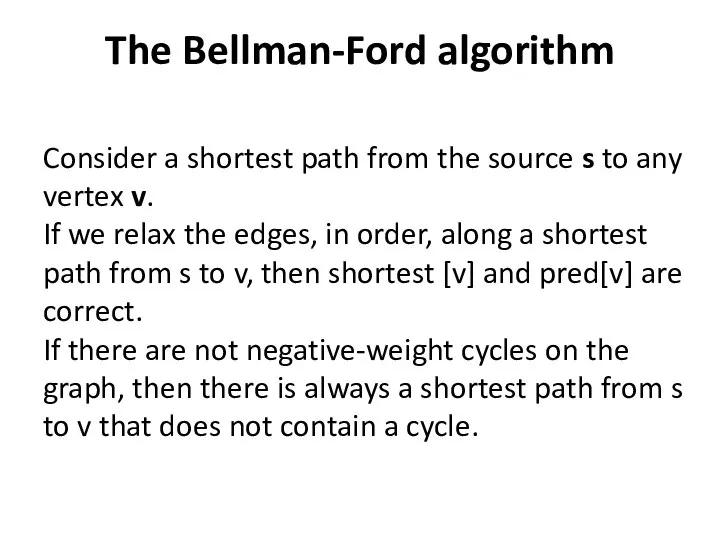
- 7. The Bellman-Ford algorithm Consider a shortest path from the source s to any vertex v. If
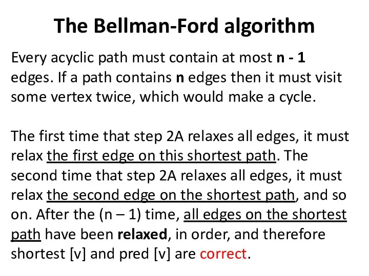
- 8. The Bellman-Ford algorithm Every acyclic path must contain at most n - 1 edges. If a
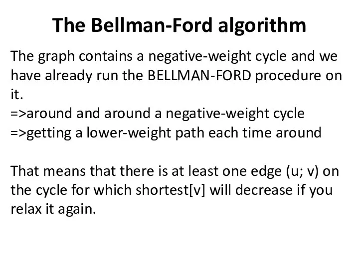
- 9. The Bellman-Ford algorithm The graph contains a negative-weight cycle and we have already run the BELLMAN-FORD
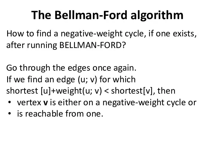
- 10. The Bellman-Ford algorithm How to find a negative-weight cycle, if one exists, after running BELLMAN-FORD? Go
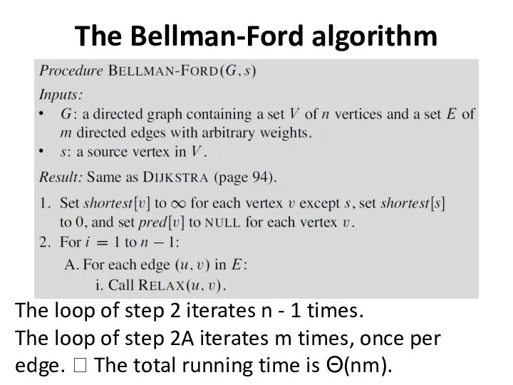
- 12. The Bellman-Ford algorithm The loop of step 2 iterates n - 1 times. The loop of
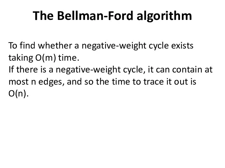
- 13. The Bellman-Ford algorithm To find whether a negative-weight cycle exists taking O(m) time. If there is
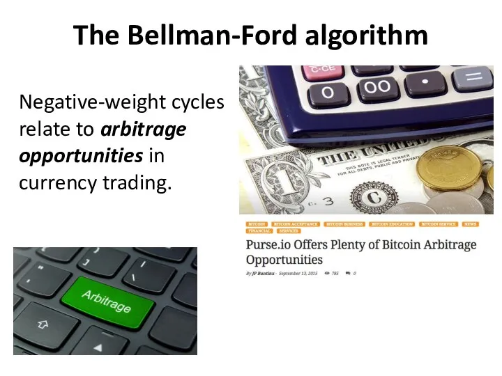
- 14. The Bellman-Ford algorithm Negative-weight cycles relate to arbitrage opportunities in currency trading.
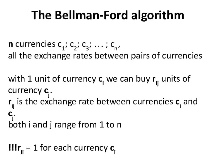
- 15. The Bellman-Ford algorithm n currencies c1; c2; c3; … ; cn, all the exchange rates between
- 16. The Bellman-Ford algorithm
- 17. The Bellman-Ford algorithm
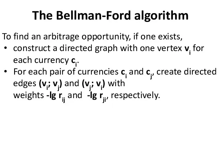
- 18. The Bellman-Ford algorithm To find an arbitrage opportunity, if one exists, construct a directed graph with
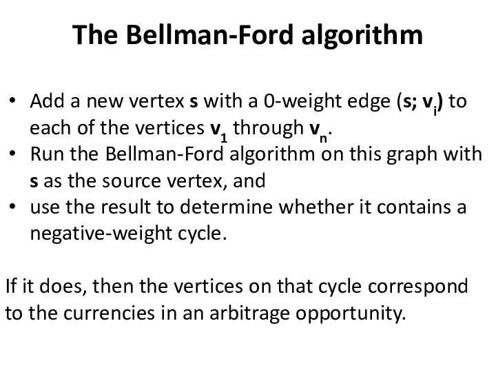
- 19. The Bellman-Ford algorithm Add a new vertex s with a 0-weight edge (s; vi) to each
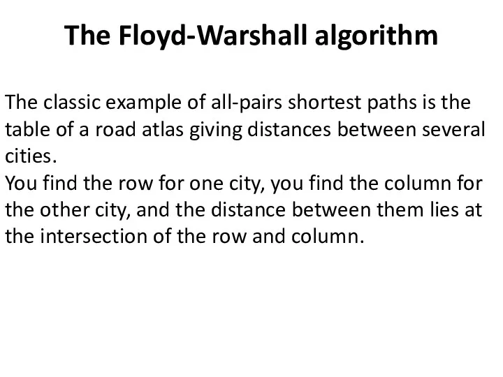
- 20. The Floyd-Warshall algorithm The classic example of all-pairs shortest paths is the table of a road
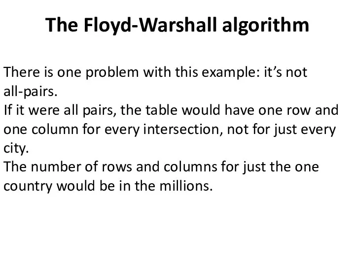
- 21. The Floyd-Warshall algorithm There is one problem with this example: it’s not all-pairs. If it were
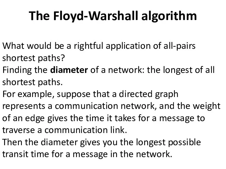
- 22. The Floyd-Warshall algorithm What would be a rightful application of all-pairs shortest paths? Finding the diameter
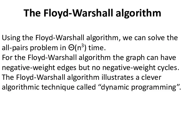
- 23. The Floyd-Warshall algorithm Using the Floyd-Warshall algorithm, we can solve the all-pairs problem in Θ(n3) time.
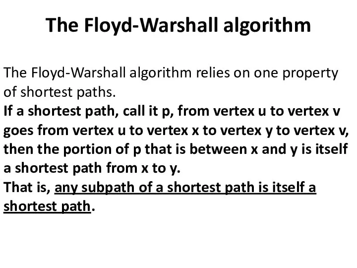
- 24. The Floyd-Warshall algorithm The Floyd-Warshall algorithm relies on one property of shortest paths. If a shortest
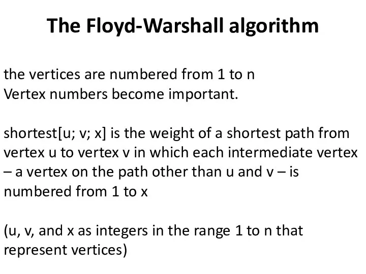
- 25. The Floyd-Warshall algorithm the vertices are numbered from 1 to n Vertex numbers become important. shortest[u;
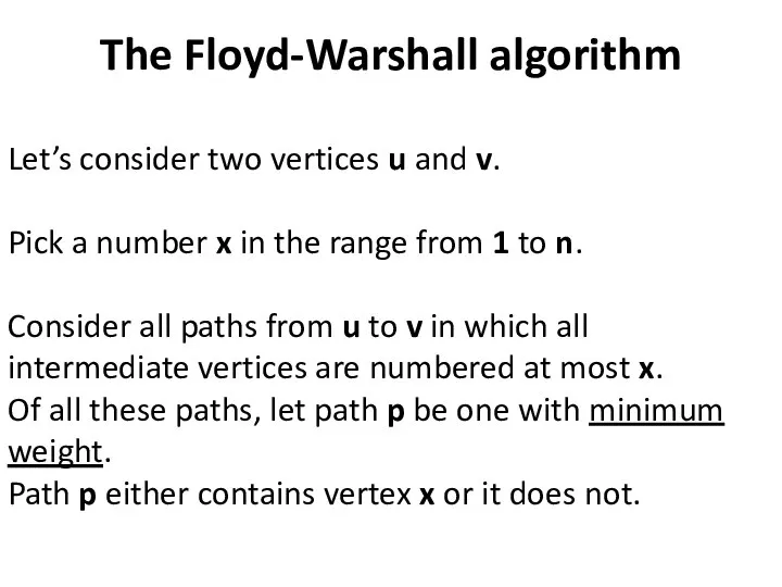
- 26. The Floyd-Warshall algorithm Let’s consider two vertices u and v. Pick a number x in the
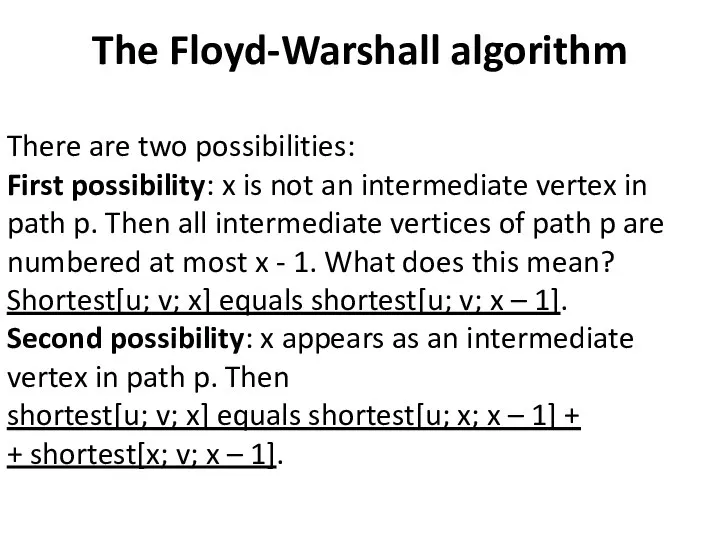
- 27. The Floyd-Warshall algorithm There are two possibilities: First possibility: x is not an intermediate vertex in
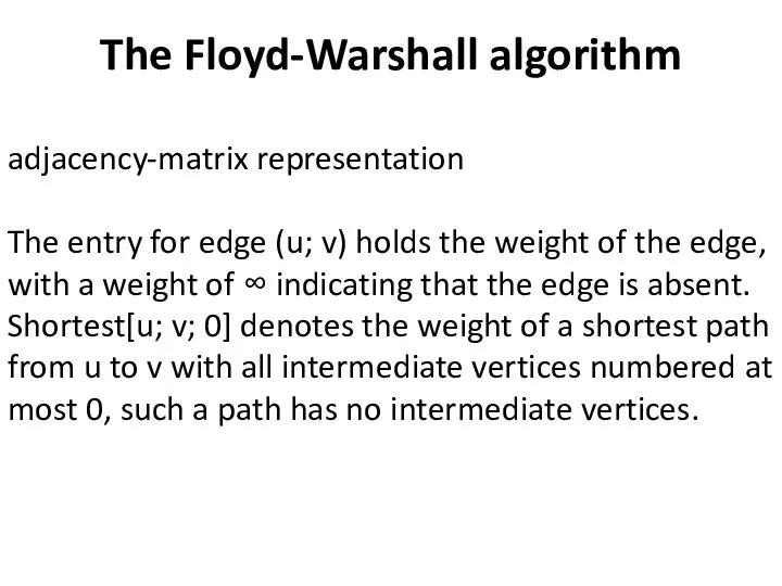
- 28. The Floyd-Warshall algorithm adjacency-matrix representation The entry for edge (u; v) holds the weight of the
- 29. The Floyd-Warshall algorithm computes shortest[u; v; x] values => x=1 computes shortest[u; v; x] values =>
- 31. The Floyd-Warshall algorithm example shortest[2; 4; 0] is 1, because we can get from vertex 2
- 32. The Floyd-Warshall algorithm pred[u; v; 0] values
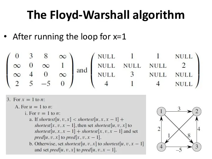
- 33. The Floyd-Warshall algorithm After running the loop for x=1
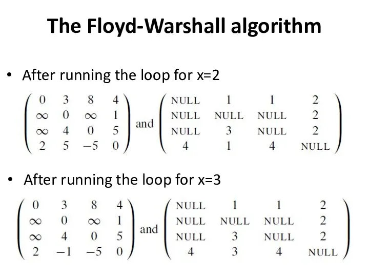
- 34. The Floyd-Warshall algorithm After running the loop for x=2 After running the loop for x=3
- 35. The Floyd-Warshall algorithm shortest[u; v; 4] and pred[u; v; 4] values
- 37. Скачать презентацию
The Bellman-Ford algorithm
1958
1962
The Bellman-Ford algorithm
1958
1962
The Bellman-Ford algorithm
The Bellman-Ford algorithm
The Bellman-Ford algorithm
the fixed order: (t; x); (t; y); (t; z);
The Bellman-Ford algorithm
the fixed order: (t; x); (t; y); (t; z);
The Bellman-Ford algorithm
Parts (b) through (e) show the situation after each
The Bellman-Ford algorithm
Parts (b) through (e) show the situation after each
The Bellman-Ford algorithm
The shortest and pred values in part (e) are
The Bellman-Ford algorithm
The shortest and pred values in part (e) are
The Bellman-Ford algorithm
Consider a shortest path from the source s to
The Bellman-Ford algorithm
Consider a shortest path from the source s to
The Bellman-Ford algorithm
Every acyclic path must contain at most n -
The Bellman-Ford algorithm
Every acyclic path must contain at most n -
The Bellman-Ford algorithm
The graph contains a negative-weight cycle and we have
The Bellman-Ford algorithm
The graph contains a negative-weight cycle and we have
The Bellman-Ford algorithm
How to find a negative-weight cycle, if one exists,
The Bellman-Ford algorithm
How to find a negative-weight cycle, if one exists,
The Bellman-Ford algorithm
The loop of step 2 iterates n - 1
The Bellman-Ford algorithm
The loop of step 2 iterates n - 1
The Bellman-Ford algorithm
To find whether a negative-weight cycle exists taking O(m)
The Bellman-Ford algorithm
To find whether a negative-weight cycle exists taking O(m)
The Bellman-Ford algorithm
Negative-weight cycles relate to arbitrage opportunities in currency trading.
The Bellman-Ford algorithm
Negative-weight cycles relate to arbitrage opportunities in currency trading.
The Bellman-Ford algorithm
n currencies c1; c2; c3; … ; cn,
all
The Bellman-Ford algorithm
n currencies c1; c2; c3; … ; cn,
all
The Bellman-Ford algorithm
The Bellman-Ford algorithm
The Bellman-Ford algorithm
The Bellman-Ford algorithm
The Bellman-Ford algorithm
To find an arbitrage opportunity, if one exists,
construct
The Bellman-Ford algorithm
To find an arbitrage opportunity, if one exists,
construct
The Bellman-Ford algorithm
Add a new vertex s with a 0-weight edge
The Bellman-Ford algorithm
Add a new vertex s with a 0-weight edge
The Floyd-Warshall algorithm
The classic example of all-pairs shortest paths is
The Floyd-Warshall algorithm
The classic example of all-pairs shortest paths is
The Floyd-Warshall algorithm
There is one problem with this example: it’s
The Floyd-Warshall algorithm
There is one problem with this example: it’s
The Floyd-Warshall algorithm
What would be a rightful application of all-pairs
The Floyd-Warshall algorithm
What would be a rightful application of all-pairs
The Floyd-Warshall algorithm
Using the Floyd-Warshall algorithm, we can solve the
The Floyd-Warshall algorithm
Using the Floyd-Warshall algorithm, we can solve the
The Floyd-Warshall algorithm
The Floyd-Warshall algorithm relies on one property of
The Floyd-Warshall algorithm
The Floyd-Warshall algorithm relies on one property of
The Floyd-Warshall algorithm
the vertices are numbered from 1 to n
Vertex
The Floyd-Warshall algorithm
the vertices are numbered from 1 to n
Vertex
The Floyd-Warshall algorithm
Let’s consider two vertices u and v.
Pick
The Floyd-Warshall algorithm
Let’s consider two vertices u and v.
Pick
The Floyd-Warshall algorithm
There are two possibilities:
First possibility: x is not
The Floyd-Warshall algorithm
There are two possibilities:
First possibility: x is not
The Floyd-Warshall algorithm
adjacency-matrix representation
The entry for edge (u; v) holds
The Floyd-Warshall algorithm
adjacency-matrix representation
The entry for edge (u; v) holds
![The Floyd-Warshall algorithm computes shortest[u; v; x] values => x=1 computes](/_ipx/f_webp&q_80&fit_contain&s_1440x1080/imagesDir/jpg/1464658/slide-28.jpg)
The Floyd-Warshall algorithm
computes shortest[u; v; x] values => x=1
computes shortest[u;
The Floyd-Warshall algorithm
computes shortest[u; v; x] values => x=1
computes shortest[u;
![The Floyd-Warshall algorithm example shortest[2; 4; 0] is 1, because we](/_ipx/f_webp&q_80&fit_contain&s_1440x1080/imagesDir/jpg/1464658/slide-30.jpg)
The Floyd-Warshall algorithm
example
shortest[2; 4; 0] is 1, because we can
The Floyd-Warshall algorithm
example
shortest[2; 4; 0] is 1, because we can
![The Floyd-Warshall algorithm pred[u; v; 0] values](/_ipx/f_webp&q_80&fit_contain&s_1440x1080/imagesDir/jpg/1464658/slide-31.jpg)
The Floyd-Warshall algorithm
pred[u; v; 0] values
The Floyd-Warshall algorithm
pred[u; v; 0] values
The Floyd-Warshall algorithm
After running the loop for x=1
The Floyd-Warshall algorithm
After running the loop for x=1
The Floyd-Warshall algorithm
After running the loop for x=2
After running the
The Floyd-Warshall algorithm
After running the loop for x=2
After running the
![The Floyd-Warshall algorithm shortest[u; v; 4] and pred[u; v; 4] values](/_ipx/f_webp&q_80&fit_contain&s_1440x1080/imagesDir/jpg/1464658/slide-34.jpg)
The Floyd-Warshall algorithm
shortest[u; v; 4] and pred[u; v; 4] values
The Floyd-Warshall algorithm
shortest[u; v; 4] and pred[u; v; 4] values
 Наибольший общий делитель
 Аттестационная работа. Эссе о включении учащихся в проектную деятельность на уроках математики
 Объем прямоугольного параллелепипеда
 Устный счет. Арифметический корень натуральной степени
 Теорема Пифагора (теорема нимфы, теорема невесты)
 Основные понятия и определения графа и его элементов
 Задачи на проценты 2
 Серединный перпендикуляр
 Аттестационная работа. Математическое общество учащихся Ориентир
 Решение задач по теме «Векторы»
 Булевы отношения
 Как путешествует точка? 6 класс
 Аналитическая геометрия
 Задача оптимизации
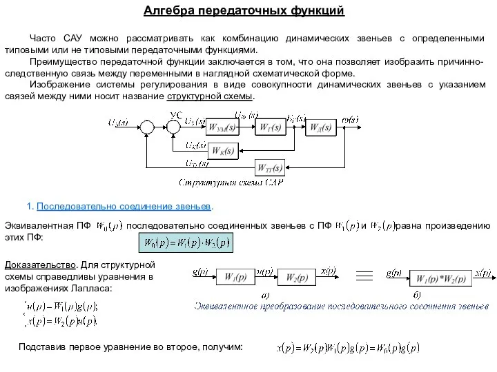 Алгебра передаточных функций
 Показатели вариации
 Презентация на тему Сложение и вычитание в пределах 20
  Математика в жизни человека Киреева Ольга и Пономарёва Анастасия ученицы 6 класса МБОУ ООШ с.Никольское.
 В царстве чисел-великанов. (6 класс)
 Решение тригонометрических уравнений функционально-графическим методом
 Графики, уравнения, неравенства
 Формула разности квадратов. 7 класс
 Шар. Задачи
 Пропорции и отношения
 Рисуем по координатам
 Сумма углов треугольника
 Система линейных уравнений с двумя переменными
 8 способов решения квадратного уравнения. 8 класс