- A combined vision-robot arm. System for material assortment

Содержание
- 2. Introduction Object Recognition via Classical Moments Control of a Robot Arm System Conclusion Contents:
- 3. In this project, an application of computer image processing to recognize various objects and the vision-based
- 4. Introduction Image Processing (Object Recognition via feature extraction, Edge Detection to define the place of the
- 5. After Hu presented moment invarients in 1962, they are widely used in many applications. Subsequently, Resis
- 6. Image Processing via Classical Moments Central Moment of an Area: Whereas; and If we calculate the
- 7. Image Processing via Classical Moments Hu moments can be found. (2) (3) (4)
- 8. Image Processing via Classical Moments (5) (6) (7) Six of these invariants are invariable if the
- 9. Image Processing via Classical Moments Zernike Moments: Zernike polynomials, form a complete orthogonal set over the
- 10. Image Processing via Classical Moments Zernike moments of order p with repitation q for a digital
- 11. Image Processing via Classical Moments Orthogonal Fourier-Mellin Moments: r is the length of the vector from
- 12. Image Processing via Classical Moments The magnitude of Hu moments, OFMMs and ZMs are rotation, translation
- 13. Image Processing via Classical Moments Light Shields (on both sides) CCD Camera (connected to the grabber
- 14. Image Processing via Classical Moments Trigerring Line Boundary Lines Object Direction Object Conveyor Band CCD Camera
- 15. Image Processing via Classical Moments In this project, four types of image processing techniques are used:
- 16. Image Processing via Classical Moments Image Data Reduction a. Digital Conversion: It reduces the number of
- 17. Image Processing via Classical Moments 2. Segmentation a. Edge Detection In Edge Detection it is considered
- 18. Image Processing via Classical Moments Some examples of Canny Edge Detection Algorithym can be seen below
- 19. Image Processing via Classical Moments 2. Segmentation a. Edge Detection b. Tresholding Tresholding is a binary
- 20. Image Processing via Classical Moments 2. Segmentation a. Edge Detection b. Tresholding Max{[((k-j)2*h[k])] | (0 J:
- 21. Image Processing via Classical Moments Images of some of the objects, tresholded images and histograms of
- 22. Image Processing via Classical Moments 3. Feature Extraction Hu moments, Legendre moments, ortogonal moments, geometrical moments,
- 23. Image Processing via Classical Moments 4. Object Recognition Object Recognition process can be defined as labeling
- 24. Robot Arm System and Control Motor # 5 Motor # 4 Motor # 3 Motor #
- 25. Robot Arm System and Control First, kinematic analysis and “link table “ of the revolute jointed
- 26. Robot Arm System and Control Second step in forward kinematics is to construct a table to
- 27. Robot Arm System and Control Transformation matrices according to table are,
- 28. Robot Arm System and Control In deriving the kinematical equations, we formed the product of link
- 29. Robot Arm System and Control Px , Py, Pz, can be found with respect to the
- 30. Robot Arm System and Control Before the path control applications, the position following capability of the
- 31. Robot Arm System and Control While planning a trajectory, first two or more points should be
- 32. Robot Arm System and Control After defining these angles, the trajectory of a joint can be
- 33. Robot Arm System and Control As an example the trajectory and parameters of the manipulator are
- 34. Robot Arm System and Control By this table, we can easily determine the needed time of
- 35. After theoretical study, to test the performance of the presented algorithym, an application mechanism is prepared
- 37. Скачать презентацию

Introduction
Object Recognition via Classical Moments
Control of a Robot
Introduction
Object Recognition via Classical Moments
Control of a Robot

In this project, an application of computer image processing to
In this project, an application of computer image processing to

Introduction
Image Processing
(Object Recognition
via feature extraction,
Edge Detection to define
Introduction
Image Processing
(Object Recognition
via feature extraction,
Edge Detection to define

After Hu presented moment invarients in 1962, they are widely
After Hu presented moment invarients in 1962, they are widely

Image Processing via Classical Moments
Central Moment of an Area:
Whereas;
and
If we
Image Processing via Classical Moments
Central Moment of an Area:
Whereas;
and
If we

Image Processing via Classical Moments
Hu moments can be found.
(2)
(3)
(4)
Image Processing via Classical Moments
Hu moments can be found.
(2)
(3)
(4)

Image Processing via Classical Moments
(5)
(6)
(7)
Six of these invariants are invariable if
Image Processing via Classical Moments
(5)
(6)
(7)
Six of these invariants are invariable if

Image Processing via Classical Moments
Zernike Moments:
Zernike polynomials, form a complete orthogonal
Image Processing via Classical Moments
Zernike Moments:
Zernike polynomials, form a complete orthogonal

Image Processing via Classical Moments
Zernike moments of order p with repitation
Image Processing via Classical Moments
Zernike moments of order p with repitation

Image Processing via Classical Moments
Orthogonal Fourier-Mellin Moments:
r is the length
Image Processing via Classical Moments
Orthogonal Fourier-Mellin Moments:
r is the length

Image Processing via Classical Moments
The magnitude of Hu moments, OFMMs and
Image Processing via Classical Moments
The magnitude of Hu moments, OFMMs and

Image Processing via Classical Moments
Light Shields
(on both sides)
CCD Camera
(connected to the
Image Processing via Classical Moments
Light Shields
(on both sides)
CCD Camera
(connected to the

Image Processing via Classical Moments
Trigerring Line
Boundary Lines
Object Direction
Object
Conveyor Band
CCD Camera
Image Processing via Classical Moments
Trigerring Line
Boundary Lines
Object Direction
Object
Conveyor Band
CCD Camera

Image Processing via Classical Moments
In this project, four types of
Image Processing via Classical Moments
In this project, four types of

Image Processing via Classical Moments
Image Data Reduction
a. Digital Conversion:
It reduces
Image Processing via Classical Moments
Image Data Reduction
a. Digital Conversion:
It reduces

Image Processing via Classical Moments
2. Segmentation
a. Edge Detection
In Edge Detection
Image Processing via Classical Moments
2. Segmentation
a. Edge Detection
In Edge Detection

Image Processing via Classical Moments
Some examples of Canny Edge Detection Algorithym
Image Processing via Classical Moments
Some examples of Canny Edge Detection Algorithym

Image Processing via Classical Moments
2. Segmentation
a. Edge Detection
b. Tresholding
Tresholding is
Image Processing via Classical Moments
2. Segmentation
a. Edge Detection
b. Tresholding
Tresholding is
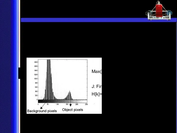
Image Processing via Classical Moments
2. Segmentation
a. Edge Detection
b. Tresholding
Max{[((k-j)2*h[k])] |
Image Processing via Classical Moments
2. Segmentation
a. Edge Detection
b. Tresholding
Max{[((k-j)2*h[k])] |

Image Processing via Classical Moments
Images of some of the objects, tresholded
Image Processing via Classical Moments
Images of some of the objects, tresholded

Image Processing via Classical Moments
3. Feature Extraction
Hu moments, Legendre moments, ortogonal
Image Processing via Classical Moments
3. Feature Extraction
Hu moments, Legendre moments, ortogonal

Image Processing via Classical Moments
4. Object Recognition
Object Recognition process can be
Image Processing via Classical Moments
4. Object Recognition
Object Recognition process can be

Robot Arm System and Control
Motor # 5
Motor # 4
Motor
Robot Arm System and Control
Motor # 5
Motor # 4
Motor

Robot Arm System and Control
First, kinematic analysis and “link
Robot Arm System and Control
First, kinematic analysis and “link

Robot Arm System and Control
Second step in forward kinematics
Robot Arm System and Control
Second step in forward kinematics

Robot Arm System and Control
Transformation matrices according to table
Robot Arm System and Control
Transformation matrices according to table

Robot Arm System and Control
In deriving the kinematical equations,
Robot Arm System and Control
In deriving the kinematical equations,

Robot Arm System and Control
Px , Py, Pz, can
Robot Arm System and Control
Px , Py, Pz, can

Robot Arm System and Control
Before the path control applications,
Robot Arm System and Control
Before the path control applications,

Robot Arm System and Control
While planning a trajectory, first
Robot Arm System and Control
While planning a trajectory, first

Robot Arm System and Control
After defining these angles, the
Robot Arm System and Control
After defining these angles, the
Robot Arm System and Control
As an example the trajectory
Robot Arm System and Control
As an example the trajectory

Robot Arm System and Control
By this table, we can
Robot Arm System and Control
By this table, we can

After theoretical study, to test the performance of the presented
After theoretical study, to test the performance of the presented
 Кинетические свойства радиоматериалов
  Module 8. Regular Expressions
 Ирина Петровна Токмакова. Жизнь и творчество
 Дизайн и вёрстка (05)
 Ацтеки
  ПЯВУ. Основы программирования. Лекция 8. Алгоритм Евклида. “Решето” Эратосфена
 Управление персоналом
 Площадь прямоугольника Презентация к уроку математики во 2 классе учителя МОУ «СОШ п. Бурасы Новобурасского района Саратовской о
 Увеличение числа в 10,100,1000 раз. Путешествие по городу.
 Международная интеграция
 МИНИМИЗАЦИЯ ПЕРЕКЛЮЧАТЕЛЬНЫХ ФУНКЦИЙ ПО КАРТАМ КАРНО
 Адвокатура. Задача каждого адвоката и адвокатуры в целом
 01.12 Номинация
 Канада
 от почтового ящика до дополненной реальности
  Презентация Налоговые вычеты
 Презентация "Художественное описание картины Н.П. Крымова «Зимний вечер»" - скачать презентации по МХК
 Некоузская средняя общеобразовательная школа, 2006 год
 Мысли, несущие силу и исцеление
 Проектирование административно-бытовых корпусов промышленного здания
 Пожарная техника
 Учитель МХК – Рогудеева Лилия Анатольевна Symbols of the USA Символы США
 Развитие системы социальной защиты населения в Республике Казахстан
 Азаматтық іс жүргізу мерзімдері
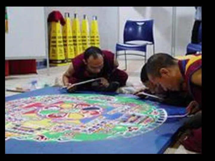 Мандала - тибетский символ божественного мира
 Обеспечение уплаты таможенных платежей (поручительство) Подготовили: Шунайлова Жанна, Епифанова Евгения
 Сущность и принципы территориального общественного самоуправления (ТОС)
 Презентация Внешнеэкономические операции и сделки