- Viscoelasticity

Содержание
- 3. Background In the nineteenth century, physicists such as Maxwell, Boltzmann, and Kelvin researched and experimented with
- 5. Types Linear viscoelasticity is when the function is separable in both creep response and load. All
- 6. Dynamic modulus Viscoelasticity is studied using dynamic mechanical analysis, applying a small oscillatory stress and measuring
- 7. Constitutive models of linear viscoelasticity Viscoelastic materials, such as amorphous polymers, semicrystalline polymers, biopolymers and even
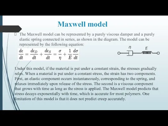
- 8. Maxwell model The Maxwell model can be represented by a purely viscous damper and a purely
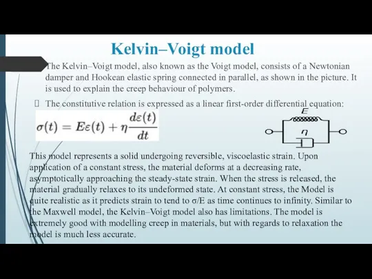
- 9. Kelvin–Voigt model The Kelvin–Voigt model, also known as the Voigt model, consists of a Newtonian damper
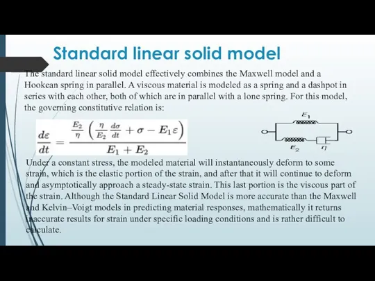
- 10. Standard linear solid model The standard linear solid model effectively combines the Maxwell model and a
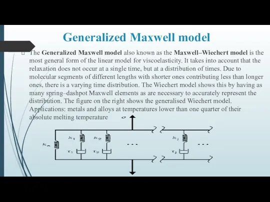
- 11. Generalized Maxwell model The Generalized Maxwell model also known as the Maxwell–Wiechert model is the most
- 13. Скачать презентацию

Background
In the nineteenth century, physicists such as Maxwell, Boltzmann, and Kelvin
Background
In the nineteenth century, physicists such as Maxwell, Boltzmann, and Kelvin

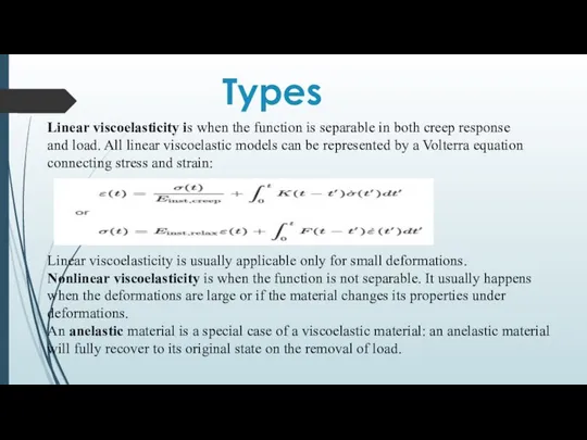
Types
Linear viscoelasticity is when the function is separable in both creep
Types
Linear viscoelasticity is when the function is separable in both creep
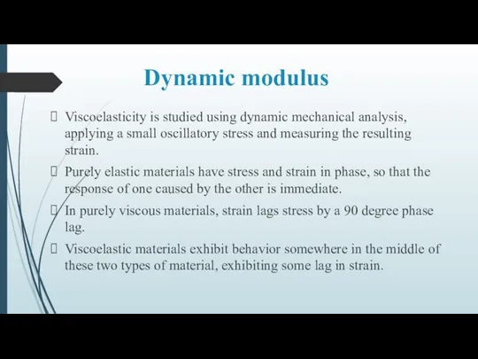
Dynamic modulus
Viscoelasticity is studied using dynamic mechanical analysis, applying a small
Dynamic modulus
Viscoelasticity is studied using dynamic mechanical analysis, applying a small
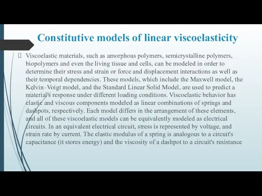
Constitutive models of linear viscoelasticity
Viscoelastic materials, such as amorphous polymers, semicrystalline
Constitutive models of linear viscoelasticity
Viscoelastic materials, such as amorphous polymers, semicrystalline
Maxwell model
The Maxwell model can be represented by a purely viscous
Maxwell model
The Maxwell model can be represented by a purely viscous
Kelvin–Voigt model
The Kelvin–Voigt model, also known as the Voigt model, consists
Kelvin–Voigt model
The Kelvin–Voigt model, also known as the Voigt model, consists
Standard linear solid model
The standard linear solid model effectively combines the
Standard linear solid model
The standard linear solid model effectively combines the
Generalized Maxwell model
The Generalized Maxwell model also known as the Maxwell–Wiechert
Generalized Maxwell model
The Generalized Maxwell model also known as the Maxwell–Wiechert
 Изменение свойств оксидов и гидроксидов металлов в зависимости от степени окисления металла
 Презентация по Химии "Атом" - скачать смотреть
  Условия движения кусков по поверхности. Грохоты
 Энтропия и уравнение состояния идеального газа
 Высокомолекулярные вещества
 Су, судың кермектілігі
 Квантовая механика- теоретическая основа современной химии
 Таза зат және қоспа. Қоспаларды бөлу әдістері. Қосылыс Рure substances and mixtures . Мethods for separating mixtures. Compound
 Периодический закон и периодическая система Д. И. Менделеева
 Биохимия гормонов
 Презентация по Химии "Химия и проблема охраны окружающей среды" - скачать смотреть бесплатно
 Химиялық өнеркәсіп
 Основы безопасности при уничтожении химического оружия
 Технология получения полиуретанов
 ЕГЭ по Химии. Задание №7
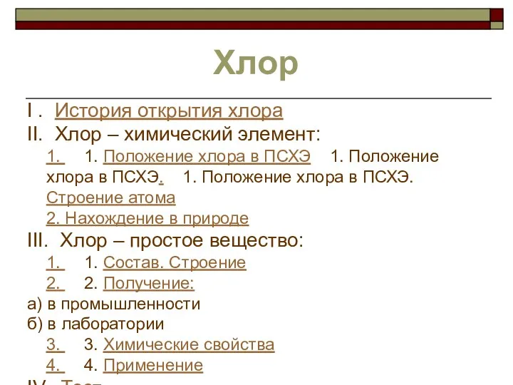 Хлор. Состав. Строение
 Вода - растворитель
 Твердые растворы Zn1,92-2хMg0,08Mn2xSiO4 и Zn1,76-2хMg0,24Mn2xSiO4: синтез и спектроскопические свойства
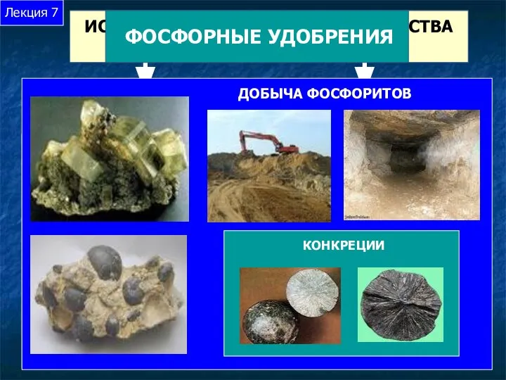 Презентация по Химии "Фосфорные удобрения" - скачать смотреть
  Математическое моделирование. Движение по градиенту
 Николаева Наталия Николаевна учитель химии МОУ «ООШ № 1 имени Бабкина Г.О.» представляет открытый урок по химии с использованием
 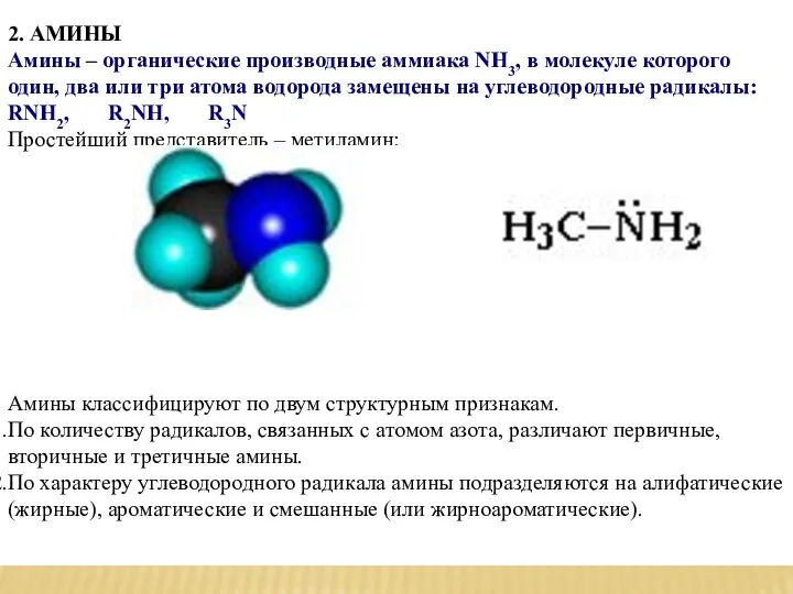 Амины. Номенклатура аминов
 Готовимся к контрольной работе по химии
 Алкины. Ацетилен
 Количества вещества
 Жиры
Жиры Альдегиды. Строение молекул
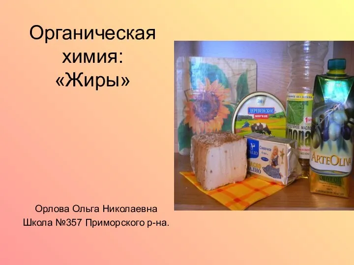 Органическая химия: «Жиры» Орлова Ольга Николаевна Школа №357 Приморского р-на.