Introduction to artificial intelligence А* Search

Август 10, 2022

Главная
Информатика
Introduction to artificial intelligence А* Search

Содержание

2. Best-First Search Review Advantages Takes advantage of domain information to guide search Greedy advance to the
3. The A* Algorithm Consider the overall cost of the solution. f(n) = g(n) + h(n) where
4. The A* Algorithm A*-Search(initial-test) ;; functions cost, h, succ, and GoalTest are defined open ;; (state,
5. A* Search: Example Travel: h(n) = distance(n, goal) 71 142 85 90 101 97 99 140
6. A* Search : Example
7. Admissible Heuristics we also require h be admissible: a heuristic h is admissible if h(n) where
8. Optimality of A* Let us assume that f is non-decreasing along each path if not, simply
9. Completeness of A* Suppose there is a goal state G with path cost f* Intuitively: since
10. UCS, BFS, Best-First, and A* f = g + h => A* Search h = 0
11. Road Map Problem s g h(s) n h(n) n’ h(n’) g(n’)
12. 8-queens State contains 8 queens on the board Successor function returns all states generated by moving
13. Heuristics : 8 Puzzle
14. 8 Puzzle Reachable state : 9!/2 = 181,440 Use of heuristics h1 : # of tiles
15. Effect of Heuristic Accuracy on Performance Well-designed heuristic have its branch close to 1 h2 dominates
17. A* summary Completeness provided finite branching factor and finite cost per operator Optimality provided we use
18. Relax Optimality Goals: Minimizing search cost Satisficing solution, i.e. bounded error in the solution f(s) =
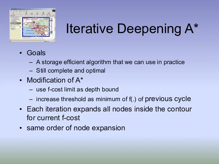
19. Iterative Deepening A* Goals A storage efficient algorithm that we can use in practice Still complete
20. IDA* Algorithm IDA* (state,h) returns solution f-limit loop do solution, f-limit ? DFS-Contour(state, f-limit) if solution
21. IDA* Properties Complete: if shortest path fits into memory Optimal: if shortest optimal path fits into
23. Скачать презентацию

Слайд 2

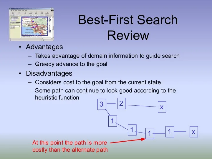
Best-First Search Review
Advantages
Takes advantage of domain information to guide search
Greedy advance

to the goal
Disadvantages
Considers cost to the goal from the current state
Some path can continue to look good according to the heuristic function

At this point the path is more
costly than the alternate path

Слайд 3

The A* Algorithm
Consider the overall cost of the solution.
f(n) = g(n)

+ h(n) where g(n) is the path cost to node n
think of f(n) as an estimate of the cost of the best solution going through the node n

Слайд 4

The A* Algorithm
A*-Search(initial-test) ;; functions cost, h, succ, and GoalTest are

defined open <- MakePriorityQueue(initial-state, NIL, 0, h(initial-state), h(initial-state))
;; (state, parent, g, h, f)
while (not(empty(open)))
node ? pop(open), state ? node-state(node)
closed ? push (closed, node)
if GoalTest(state) succeeds return node
for each child in succ(state)
new-cost ? node-g(node) + cost(state,child)
if child in open
if new-cost < g value of child
update(open, child, node, new-cost, h(child), new-cost+h(child))
elseif child in closed
if new-cost < g value of child
insert(open, child, node, new-cost, h(child), new-cost+h(child))
delete(closed,child)
else
open ? push(child, node, new-cost, h(child), new-cost+h(child))
return failure

Слайд 5

A* Search: Example
Travel: h(n) = distance(n, goal)
71
142
85
90
101
97
99
140
138
146
120
75
70
111
118
75
211
151
86
98
92
87
80

Слайд 6

A* Search : Example

Слайд 7

Admissible Heuristics
we also require h be admissible:
a heuristic h is

admissible if h(n) < h*(n) for all nodes n,
where h* is the actual cost of the optimal path from n to the goal
Examples:
travel distance straight line distance must be shorter than actual travel path
tiles out of place each move can reorder at most one tile distance of each out of place tile from the correct place each move moves a tile at most one place toward correct place

Слайд 8

Optimality of A*
Let us assume that f is non-decreasing along each

path
if not, simply use parent’s value
if that’s the case, we can think of A* as expanding f contours toward the goal; better heuristics make this contour more “eccentric”
Let G be an optimal goal state with path cost f*
Let G2 be a suboptimal goal state with path cost g(G2) > f*.
suppose A* picks G2 before G (A* is not optimal)
suppose n is a leaf node on the path to G when G2 is chosen
if h is admissible, then f* >= f(n)
since n was not chosen, it must be the case that f(n) >= f(G2)
therefore f* >= f(G2), but since G2 is a goal, h(G2)=0, so f* >= g(G2)
But this is a contradiction --- G2 is a better goal node than G
Thus, our supposition is false and A* is optimal.

Слайд 9

Completeness of A*
Suppose there is a goal state G with path

cost f*
Intuitively: since A* expands nodes in order of increasing f, it must eventually expand node G
If A* stops and fails
Prove by contradiction that this is impossible.
There exists a path from the initial state to the node state
Let n be the last node expanded along the solution path
n has at least one child, that child should be in the open nodes
A* does not stop until there are open list is empty (unless it finds a goal state). Contradiction.
A* is on an infinite path
Recall that cost(s1,s2) > δ
Let n be the last node expanded along the solution path
After f(n)/δ the cumulative cost of the path becomes large enough that A* will expand n. Contradiction.

Слайд 10

UCS, BFS, Best-First, and A*
f = g + h => A*

Search
h = 0 => Uniform cost search
g = 1, h = 0 => Breadth-First search
g = 0 => Best-First search

Слайд 11

Road Map Problem
s
g
h(s)
n
h(n)
n’
h(n’)
g(n’)

Слайд 12

8-queens
State contains 8 queens on the board
Successor function returns all states

generated by moving a single queen to another square in the same column (8*7 = 56 next states)
h(s) = number of queens that attack each other in state s.

H(s) = 17

H(s) = 1

Слайд 13

Heuristics : 8 Puzzle

Слайд 14

8 Puzzle
Reachable state : 9!/2 = 181,440
Use of heuristics
h1 :

# of tiles that are in the wrong position
h2 : sum of Manhattan distance

h1 = 3
h2 = 1+2+2=5

Слайд 15

Effect of Heuristic Accuracy on Performance
Well-designed heuristic have its branch close

to 1
h2 dominates h1 iff
h2(n) ≥ h1(n), ∀ n
It is always better to use a heuristic function with higher values, as long as it does not overestimate
Inventing heuristic functions
Cost of an exact solution to a relaxed problem is a good heuristic for the original problem
collection of admissible heuristics
h*(n) = max(h1(n), h2(n), …, hk(n))

Слайд 16

Слайд 17

A* summary
Completeness
provided finite branching factor and finite cost per operator

Optimality
provided we use an admissible heuristic
Time complexity
worst case is still O(bd) in some special cases we can do better for a given heuristic
Space complexity
worst case is still O(bd)

Слайд 18

Relax Optimality
Goals:
Minimizing search cost
Satisficing solution, i.e. bounded error in the solution
f(s)

= (1-w) g(s) + w h(s)
g can be thought of as the breadth first component
w = 1 => Best-First search
w = .5 => A* search
w = 0 => Uniform search

Слайд 19

Iterative Deepening A*
Goals
A storage efficient algorithm that we can use in

practice
Still complete and optimal
Modification of A*
use f-cost limit as depth bound
increase threshold as minimum of f(.) of previous cycle
Each iteration expands all nodes inside the contour for current f-cost
same order of node expansion

Слайд 20

IDA* Algorithm
IDA* (state,h) returns solution
f-limit <- h(state)
loop do
solution, f-limit ? DFS-Contour(state,

f-limit)
if solution is non-null return solution
if f-limit = ∞ return failure
end

DFS-Contour (node,f-limit) returns solution
if f (node) > f-limit return null, f(node)
if GoalTest(node) return node, f-limit
next-f ? ∞
for each node s in succ(node) do
solution, new-f ? DFS-Contour(s, f-limit)
if solution is non-null return solution, f-limit
next-f ? Min(next-f, new-f)
end
return null, next-f

Слайд 21

IDA* Properties
Complete:
if shortest path fits into memory
Optimal:
if shortest optimal path fits

into memory
Time Complexity: O(b2d)
Space Complexity: O(bd)

Introduction to artificial intelligence А* Search

Содержание

Best-First Search ReviewAdvantagesTakes advantage of domain information to guide searchGreedy advance

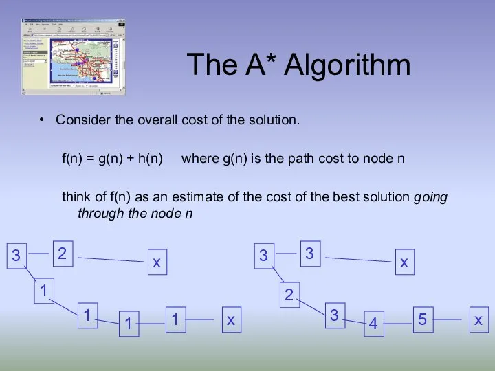
The A* AlgorithmConsider the overall cost of the solution.f(n) = g(n)

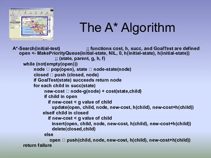
The A* AlgorithmA*-Search(initial-test) ;; functions cost, h, succ, and GoalTest are

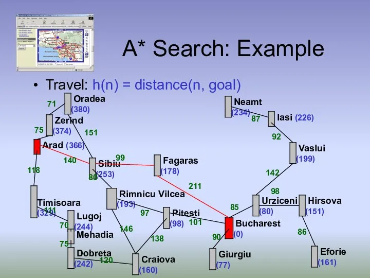
A* Search: ExampleTravel: h(n) = distance(n, goal) 71142859010197991401381461207570111118752111518698928780

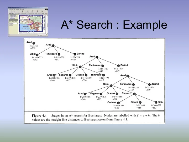
A* Search : Example

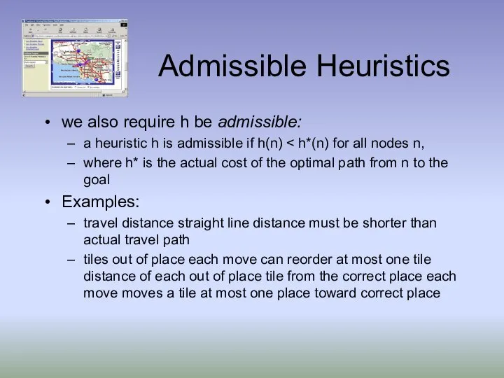
Admissible Heuristicswe also require h be admissible: a heuristic h is

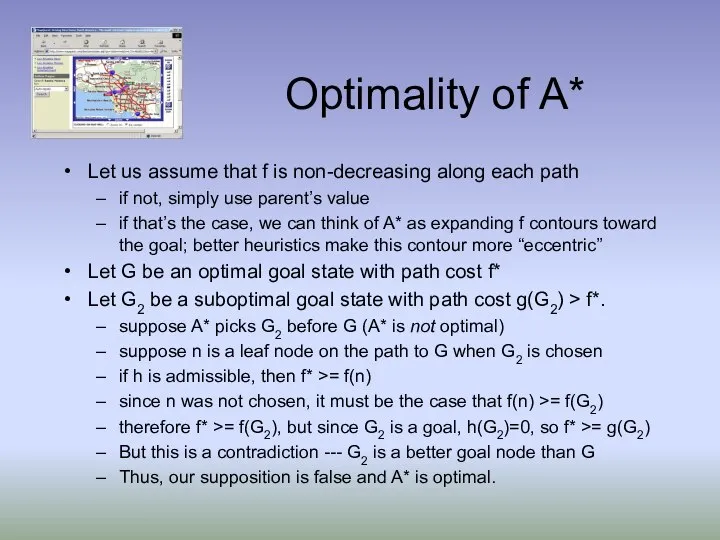
Optimality of A*Let us assume that f is non-decreasing along each

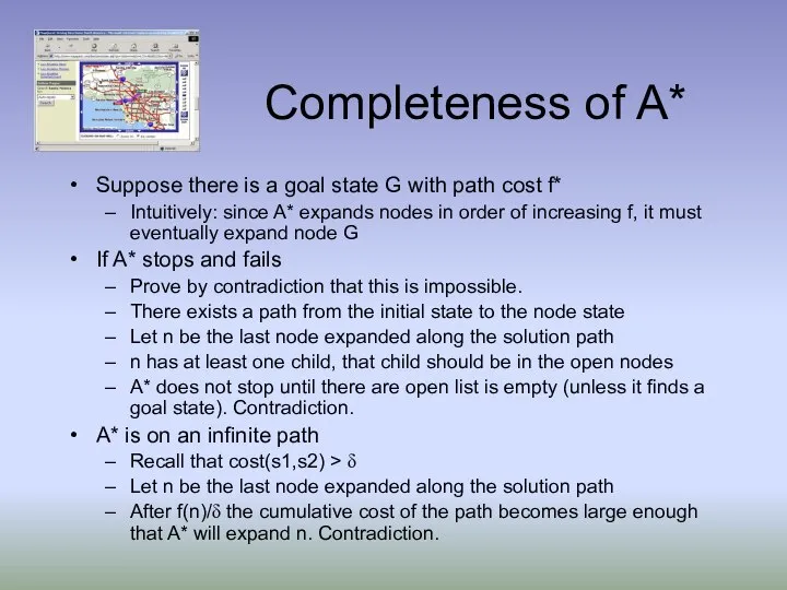
Completeness of A*Suppose there is a goal state G with path

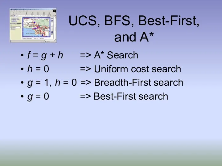
UCS, BFS, Best-First, and A*f = g + h => A*

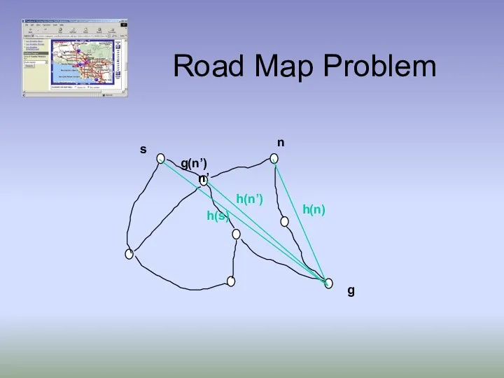
Road Map Problemsgh(s)nh(n)n’h(n’)g(n’)

8-queensState contains 8 queens on the boardSuccessor function returns all states

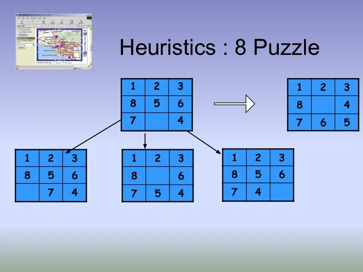
Heuristics : 8 Puzzle

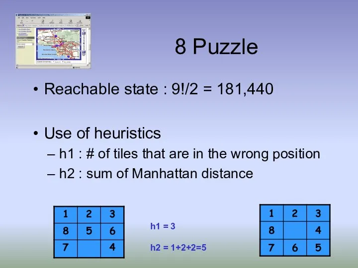
8 PuzzleReachable state : 9!/2 = 181,440Use of heuristics h1 :

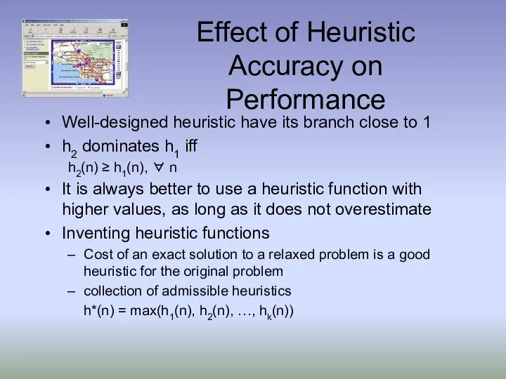
Effect of Heuristic Accuracy on PerformanceWell-designed heuristic have its branch close

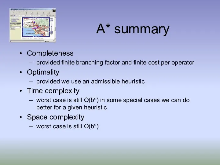
A* summaryCompleteness provided finite branching factor and finite cost per operator

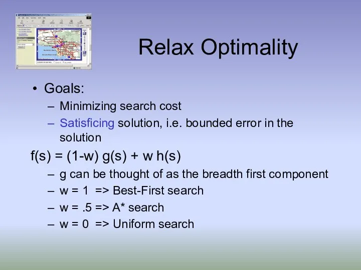
Relax OptimalityGoals:Minimizing search costSatisficing solution, i.e. bounded error in the solutionf(s)

Iterative Deepening A*GoalsA storage efficient algorithm that we can use in

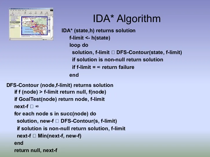
IDA* AlgorithmIDA* (state,h) returns solution f-limit <- h(state) loop do solution, f-limit ? DFS-Contour(state,

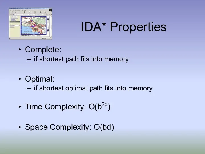
IDA* PropertiesComplete:if shortest path fits into memoryOptimal:if shortest optimal path fits

Похожие презентации