- Probabilities. Week 5 (2)

Содержание
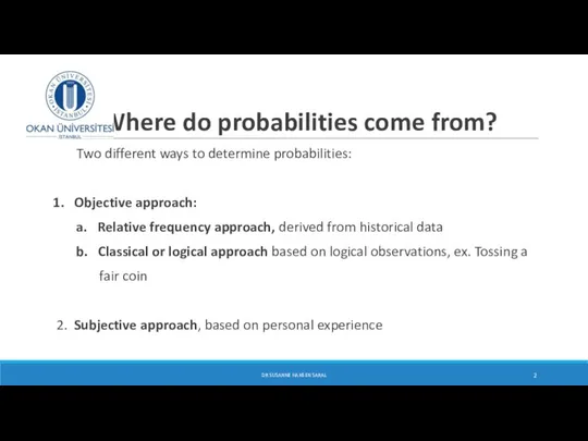
- 2. Where do probabilities come from? Two different ways to determine probabilities: 1. Objective approach: a. Relative
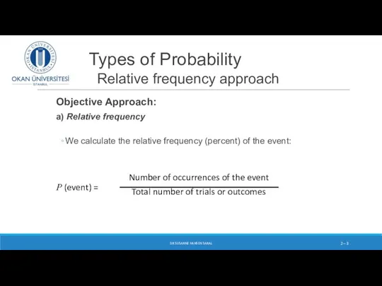
- 3. Types of Probability Relative frequency approach Objective Approach: a) Relative frequency We calculate the relative frequency
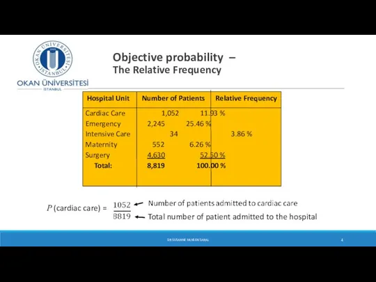
- 4. Objective probability – The Relative Frequency DR SUSANNE HANSEN SARAL Hospital Unit Number of Patients Relative
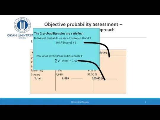
- 5. Objective probability assessment – The Relative Frequency Approach DR SUSANNE HANSEN SARAL Example: Hospital Patients by
- 6. Types of Probability Classical approach Objective Approach: DR SUSANNE HANSEN SARAL b) Classical approach: ♥ ♣
- 7. Subjective approach to assign probabilities We use the subjective approach : No possibility to use the
- 8. Types of Probability Subjective Approach: Based on the experience and judgment of the person making the
- 9. Interpreting probability No matter what method is used to assign probabilities, we interpret the probability, using
- 10. Probability rules continued Rule 1 and 2 If A is any event in the sample space
- 11. Objective probability assessment – The Relative Frequency Approach DR SUSANNE HANSEN SARAL Example: Hospital Patients by
- 12. Probability rules. Rule 3 Complement rule Suppose the probability that you win in the lottery is
- 13. Probability rules. Rule 3 Complement rule DR SUSANNE HANSEN SARAL
- 14. Probability rule 4 Multiplication rule – calculating joint probabilities Independent events DR SUSANNE HANSEN SARAL
- 15. Multiplication Rule for independent events (continued) DR SUSANNE HANSEN SARAL
- 16. Independent events Events are independent from each other when the probability of occurrence of the first
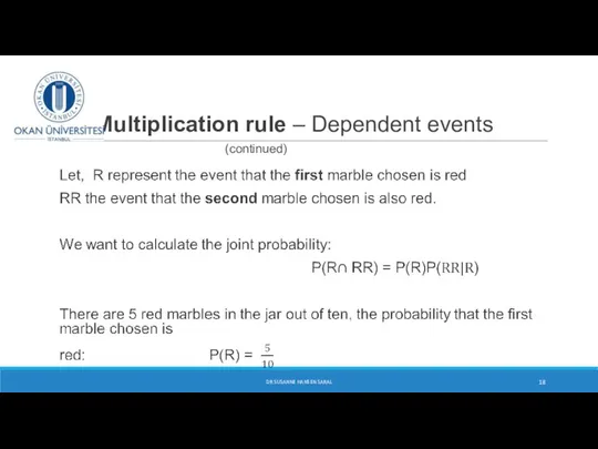
- 17. Multiplication rule – calculating joint probabilities Dependent events DR SUSANNE HANSEN SARAL
- 18. Multiplication rule – Dependent events (continued) DR SUSANNE HANSEN SARAL
- 19. Multiplication Rule - Dependent events (continued) DR SUSANNE HANSEN SARAL
- 20. Multiple choice quiz: 1 correct 3 false You are going to take a multiple choice exam.
- 21. Multiple choice quiz: 1 correct 3 false DR SUSANNE HANSEN SARAL
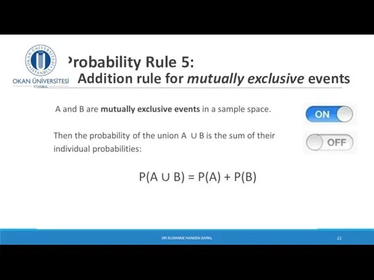
- 22. Probability Rule 5: Addition rule for mutually exclusive events DR SUSANNE HANSEN SARAL
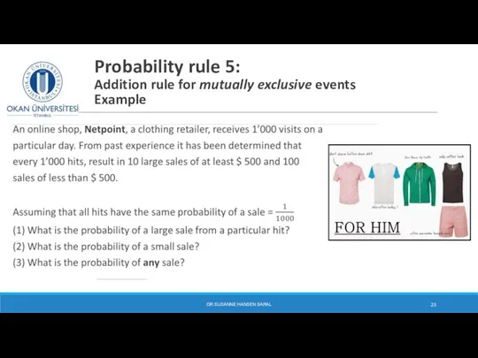
- 23. Probability rule 5: Addition rule for mutually exclusive events Example DR SUSANNE HANSEN SARAL
- 24. Addition rule of mutually exclusive events: Example – Definition of events DR SUSANNE HANSEN SARAL
- 25. Addition rule of mutually exclusive events: Example - Solution DR SUSANNE HANSEN SARAL
- 26. Addition rule of mutually exclusive events: Class exercise A corporation receives a shipment of 100 units
- 27. Probability rule 6: Addition rule for non- mutually exclusive events A∩B A B S DR SUSANNE
- 28. DR SUSANNE HANSEN SARAL Probability rule 6: Addition rule for non-mutually exclusive events
- 29. Addition rule of mutually non-exclusive events rolling a dice DR SUSANNE HANSEN SARAL Ch. 3- S
- 30. Addition rule of mutually non-exclusive events: Example: P (A U B) = P(A) + P(B) –
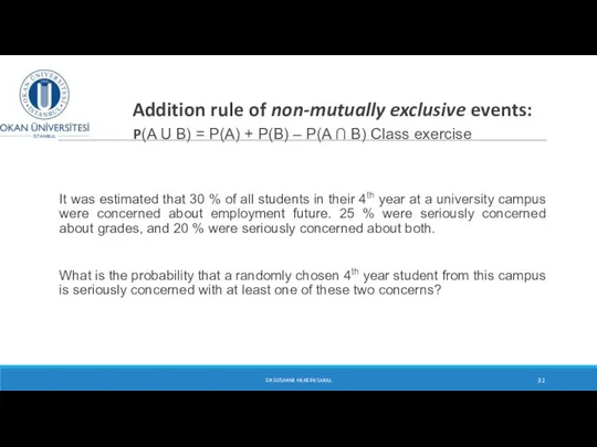
- 31. Addition rule of non-mutually exclusive events: Example: A video store owner finds that 30 % of
- 32. Addition rule of non-mutually exclusive events: P(A U B) = P(A) + P(B) – P(A ∩
- 33. Class exercise - solution DR SUSANNE HANSEN SARAL
- 34. Calculating probabilities of complex events Now we will look at how to calculate the probability of
- 35. How to calculate probabilities of intersecting events DR SUSANNE HANSEN SARAL
- 36. Drawing a Card – not mutually exclusive Draw one card from a deck of 52 playing
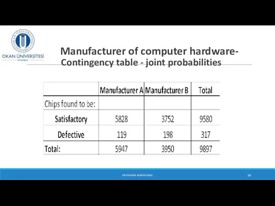
- 37. Joint probabilities - A business application A manufacturer of computer hardware buys microprocessors chips to use
- 38. Manufacturer of computer hardware- Contingency table - joint probabilities DR SUSANNE HANSEN SARAL
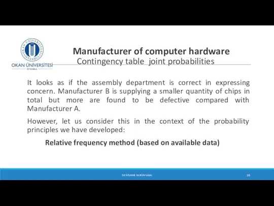
- 39. Manufacturer of computer hardware Contingency table joint probabilities It looks as if the assembly department is
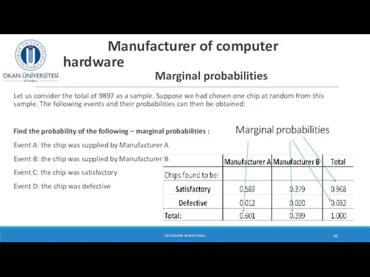
- 40. Manufacturer of computer hardware Marginal probabilities Let us consider the total of 9897 as a sample.
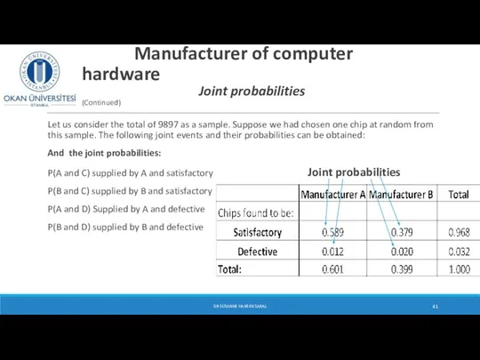
- 41. Manufacturer of computer hardware Joint probabilities (Continued) Let us consider the total of 9897 as a
- 42. Interpretation of the joint probabilities in the example The joint probability that a chip is defective
- 43. Notations for the marginal and joint events DR SUSANNE HANSEN SARAL
- 44. Marginal probabilities DR SUSANNE HANSEN SARAL
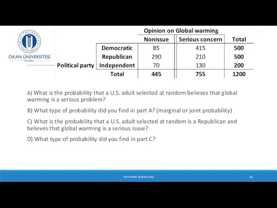
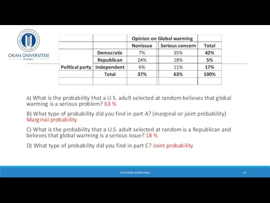
- 45. The following contingency table shows opinion about global warming among U.S. adults, broken down by political
- 46. A) What is the probability that a U.S. adult selected at random believes that global warming
- 47. A) What is the probability that a U.S. adult selected at random believes that global warming
- 49. Скачать презентацию
Where do probabilities come from?
Two different ways to determine probabilities:
1.
Where do probabilities come from?
Two different ways to determine probabilities:
1.
Types of Probability
Relative frequency approach
Objective Approach:
a) Relative frequency
We calculate
Types of Probability
Relative frequency approach
Objective Approach:
a) Relative frequency
We calculate
Objective probability –
The Relative Frequency
DR SUSANNE HANSEN SARAL
Objective probability –
The Relative Frequency
DR SUSANNE HANSEN SARAL
Objective probability assessment –
The Relative Frequency Approach
DR SUSANNE
Objective probability assessment –
The Relative Frequency Approach
DR SUSANNE
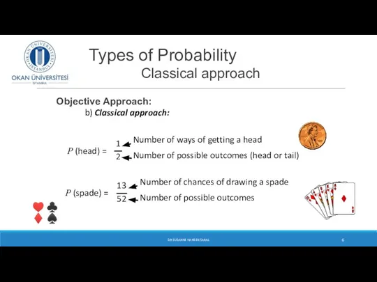
Types of Probability Classical approach
Objective Approach:
DR SUSANNE HANSEN SARAL
b)
Types of Probability Classical approach
Objective Approach:
DR SUSANNE HANSEN SARAL
b)

Subjective approach to assign probabilities
We use the subjective approach :
No
Subjective approach to assign probabilities
We use the subjective approach :
No
Types of Probability
Subjective Approach:
Based on the experience and judgment of the
Types of Probability
Subjective Approach:
Based on the experience and judgment of the
Interpreting probability
No matter what method is used to assign probabilities, we
Interpreting probability
No matter what method is used to assign probabilities, we
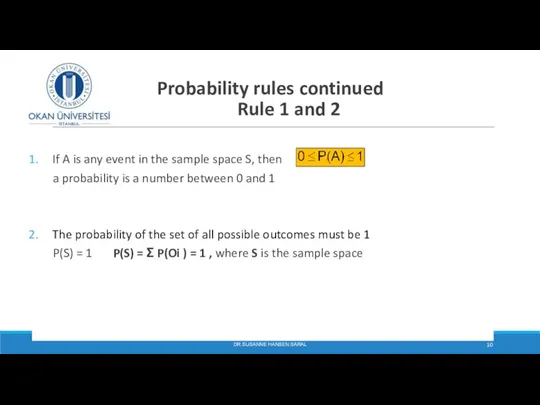
Probability rules continued
Rule 1 and 2
If A is any event
Probability rules continued
Rule 1 and 2
If A is any event

Objective probability assessment –
The Relative Frequency Approach
DR SUSANNE
Objective probability assessment –
The Relative Frequency Approach
DR SUSANNE
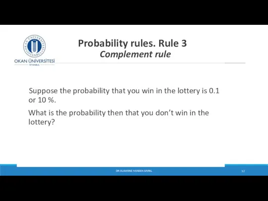
Probability rules. Rule 3
Complement rule
Suppose the probability that you win
Probability rules. Rule 3
Complement rule
Suppose the probability that you win
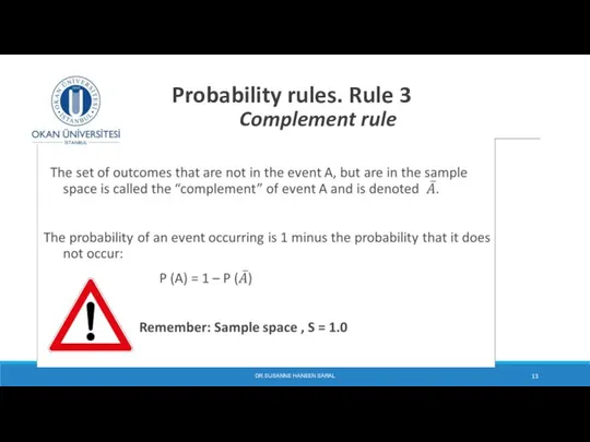
Probability rules. Rule 3
Complement rule
DR SUSANNE HANSEN SARAL
Probability rules. Rule 3
Complement rule
DR SUSANNE HANSEN SARAL
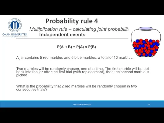
Probability rule 4
Multiplication rule – calculating joint probabilities
Independent
Probability rule 4 Multiplication rule – calculating joint probabilities Independent

Multiplication Rule for independent events (continued)
DR SUSANNE HANSEN SARAL
Multiplication Rule for independent events (continued)
DR SUSANNE HANSEN SARAL
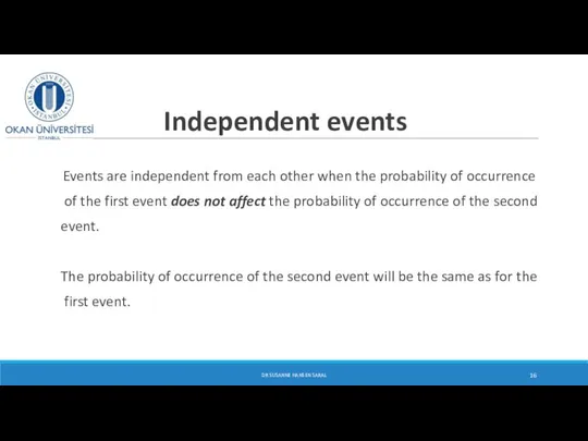
Independent events
Events are independent from each other when the
Independent events
Events are independent from each other when the

Multiplication rule – calculating joint probabilities
Dependent events
DR SUSANNE HANSEN SARAL
Multiplication rule – calculating joint probabilities
Dependent events
DR SUSANNE HANSEN SARAL
Multiplication rule – Dependent events (continued)
DR SUSANNE HANSEN SARAL
Multiplication rule – Dependent events (continued)
DR SUSANNE HANSEN SARAL

Multiplication Rule - Dependent events (continued)
DR SUSANNE HANSEN SARAL
Multiplication Rule - Dependent events (continued)
DR SUSANNE HANSEN SARAL

Multiple choice quiz: 1 correct 3 false
You are going
Multiple choice quiz: 1 correct 3 false
You are going

Multiple choice quiz: 1 correct 3 false
DR SUSANNE HANSEN SARAL
Multiple choice quiz: 1 correct 3 false
DR SUSANNE HANSEN SARAL
Probability Rule 5:
Addition rule for mutually exclusive events
DR SUSANNE
Probability Rule 5:
Addition rule for mutually exclusive events
DR SUSANNE
Probability rule 5:
Addition rule for mutually exclusive events
Example
DR SUSANNE HANSEN SARAL
Probability rule 5:
Addition rule for mutually exclusive events
Example
DR SUSANNE HANSEN SARAL
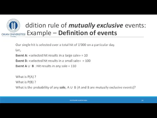
Addition rule of mutually exclusive events: Example – Definition of events
DR
Addition rule of mutually exclusive events: Example – Definition of events
DR
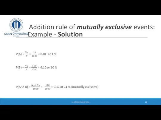
Addition rule of mutually exclusive events: Example - Solution
DR
Addition rule of mutually exclusive events: Example - Solution
DR
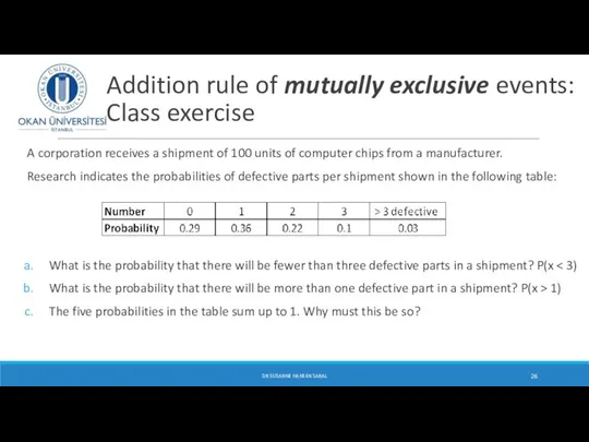
Addition rule of mutually exclusive events: Class exercise
A corporation receives
Addition rule of mutually exclusive events: Class exercise
A corporation receives
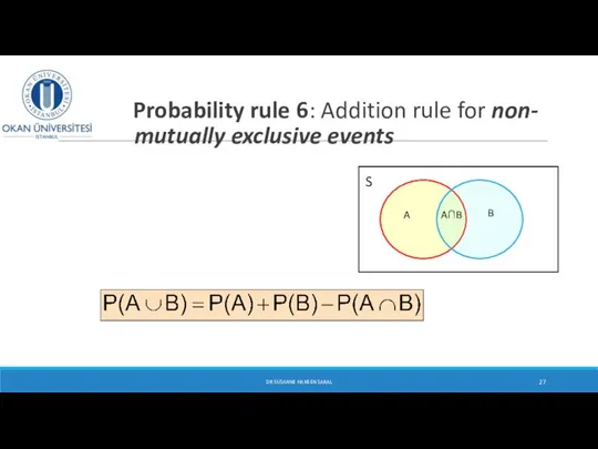
Probability rule 6: Addition rule for non-
mutually exclusive events
Probability rule 6: Addition rule for non- mutually exclusive events

DR SUSANNE HANSEN SARAL
Probability rule 6: Addition rule for non-mutually
DR SUSANNE HANSEN SARAL
Probability rule 6: Addition rule for non-mutually
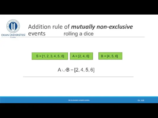
Addition rule of mutually non-exclusive events rolling a dice
DR SUSANNE HANSEN
Addition rule of mutually non-exclusive events rolling a dice
DR SUSANNE HANSEN

Addition rule of mutually non-exclusive events: Example: P (A U
Addition rule of mutually non-exclusive events: Example: P (A U

Addition rule of non-mutually exclusive events: Example:
A video store owner
Addition rule of non-mutually exclusive events: Example:
A video store owner
Addition rule of non-mutually exclusive events: P(A U B) =
Addition rule of non-mutually exclusive events: P(A U B) =
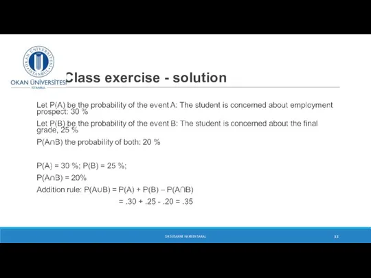
Class exercise - solution
DR SUSANNE HANSEN SARAL
Class exercise - solution
DR SUSANNE HANSEN SARAL
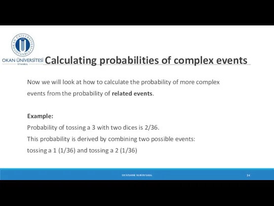
Calculating probabilities of complex events
Now we will look at how to
Calculating probabilities of complex events
Now we will look at how to
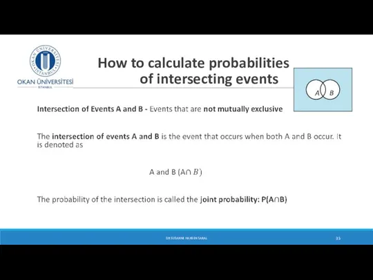
How to calculate probabilities of intersecting events
DR SUSANNE HANSEN SARAL
How to calculate probabilities of intersecting events
DR SUSANNE HANSEN SARAL

Drawing a Card – not mutually exclusive
Draw one card from a
Drawing a Card – not mutually exclusive
Draw one card from a

Joint probabilities - A business application
A manufacturer of computer hardware
Joint probabilities - A business application
A manufacturer of computer hardware
Manufacturer of computer hardware- Contingency table - joint probabilities
DR SUSANNE
Manufacturer of computer hardware- Contingency table - joint probabilities
DR SUSANNE
Manufacturer of computer hardware
Contingency table joint probabilities
It looks
Manufacturer of computer hardware
Contingency table joint probabilities
It looks
Manufacturer of computer hardware
Marginal probabilities
Let us consider the total
Manufacturer of computer hardware
Marginal probabilities
Let us consider the total
Manufacturer of computer hardware
Joint probabilities (Continued)
Let us consider the
Manufacturer of computer hardware
Joint probabilities (Continued)
Let us consider the
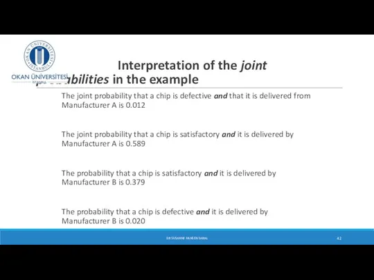
Interpretation of the joint probabilities in the example
The joint probability
Interpretation of the joint probabilities in the example
The joint probability
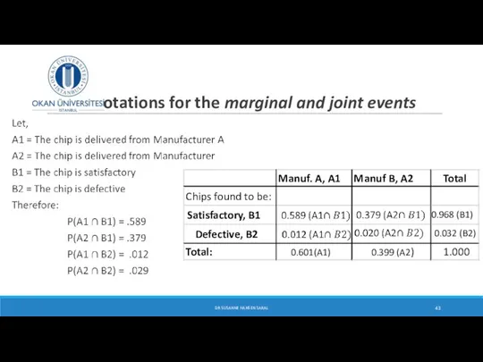
Notations for the marginal and joint events
DR SUSANNE HANSEN SARAL
Notations for the marginal and joint events
DR SUSANNE HANSEN SARAL
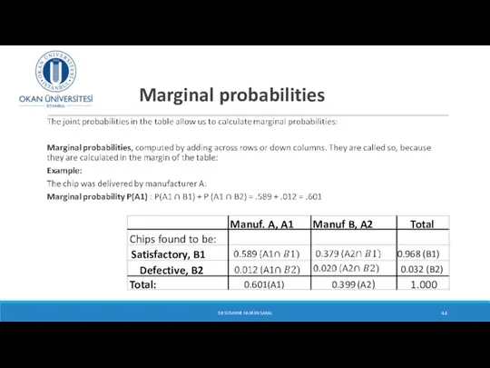
Marginal probabilities
DR SUSANNE HANSEN SARAL
Marginal probabilities
DR SUSANNE HANSEN SARAL
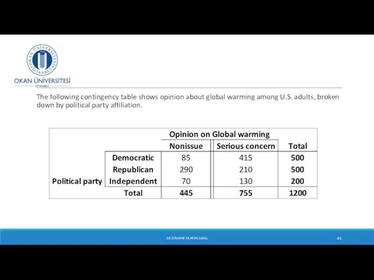
The following contingency table shows opinion about global warming among
The following contingency table shows opinion about global warming among
A) What is the probability that a U.S. adult selected
A) What is the probability that a U.S. adult selected
A) What is the probability that a U.S. adult selected
A) What is the probability that a U.S. adult selected
 В мире плоскостей
 Прямая. Луч. Отрезок
 Роль и место системного подхода
 Метод Галеркина для дифференциально-операторного уравнения третьего порядка
 Презентация на тему Призма Многогранник
 Единицы длины. 5 класс
 Моделирование зависимостей между величинами
 Решение задач на применение третьего признака равенства треугольников
 Анализ работы методического объединения точных наук за 2012-2013 учебный год. Руководитель МО точных наук: Макуева Нелла Буваевна
 Основы математического моделирования. Расчеты из первых принципов
 Аттестационная работа. Программа внеурочной деятельности для 1-4 классов Математика и конструирование
 Двухфакторный дисперсионный анализ
 Розв’язування тригонометричних рівнянь
 Сумма углов треугольника
 Правильные многогранники в природе
 Четырехугольники. Трапеция
 Показатели вариации
 Презентация на тему Логарифм числа
  Методы параметрического спектрального анализа. Введение
 Площадь треугольника. 8 класс
 Вывод формулы Герона. Геометрия 8 класс
 Описанная и вписанная окружности треугольника
 РАССТОЯНИЕ МЕЖДУ ПРЯМЫМИ В ПРОСТРАНСТВЕ
 Применение основных свойств площадей к решению задач
 Source coordinate definition by. Non-destructive assay
 Лекция 5. Транспортные задачи и задачи о назначениях Содержание лекции: Формулировка транспортной задачи Метод потенциалов Особ
 Множества. Числовые множества
 Задачи метрологии. Основные термины и определения метрологии. Системы физических величин и единиц