- Shortest Paths

Содержание
- 2. Dijkstra’s algorithm are given: source vertex s; the weight weight (u, v) of each edge (u,
- 3. Dijkstra’s algorithm
- 4. Dijkstra’s algorithm the situation at time 0 shortest[s]= 0
- 5. Dijkstra’s algorithm at time 4 shortest[y]= 4, pred[y]= s
- 6. Dijkstra’s algorithm at time 5 shortest[t]=5, pred[t]= y
- 7. Dijkstra’s algorithm at time 7 shortest[z]=7, pred[z]= y
- 8. Dijkstra’s algorithm at time 8 shortest[x]=8, pred[x]=t
- 9. Dijkstra’s algorithm Dijkstra’s algorithm works a little differently. It treats all edges the same. Dijkstra’s algorithm
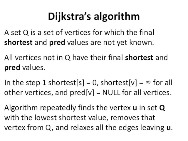
- 11. Dijkstra’s algorithm A set Q is a set of vertices for which the final shortest and
- 12. Dijkstra’s algorithm A set Q is a set of vertices for which the final shortest and
- 13. Dijkstra’s algorithm Question 1: How does the algorithm find new paths and do the relaxation? Question
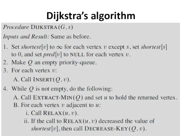
- 14. Dijkstra’s algorithm
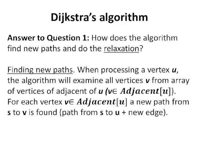
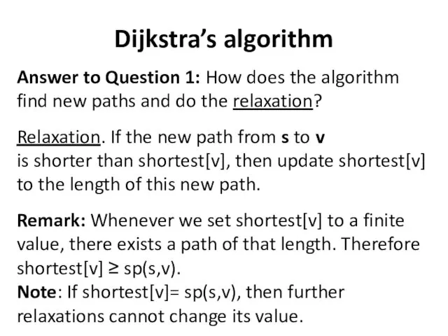
- 15. Dijkstra’s algorithm Answer to Question 1: How does the algorithm find new paths and do the
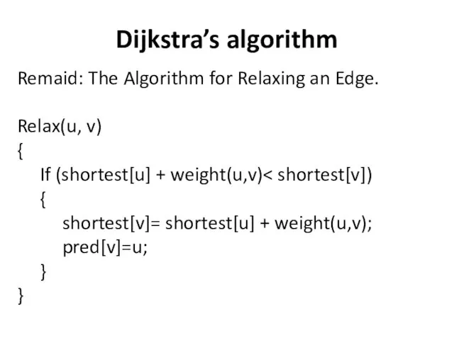
- 16. Dijkstra’s algorithm Remaid: The Algorithm for Relaxing an Edge. Relax(u, v) { If (shortest[u] + weight(u,v)
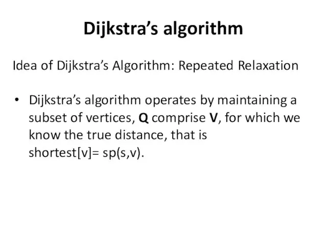
- 17. Dijkstra’s algorithm Idea of Dijkstra’s Algorithm: Repeated Relaxation Dijkstra’s algorithm operates by maintaining a subset of
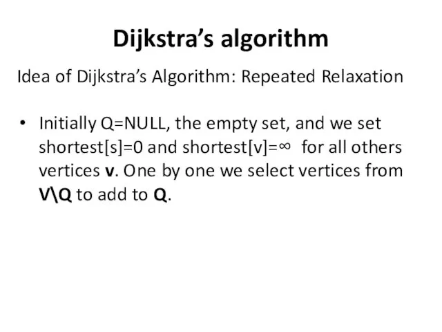
- 18. Dijkstra’s algorithm Idea of Dijkstra’s Algorithm: Repeated Relaxation Initially Q=NULL, the empty set, and we set
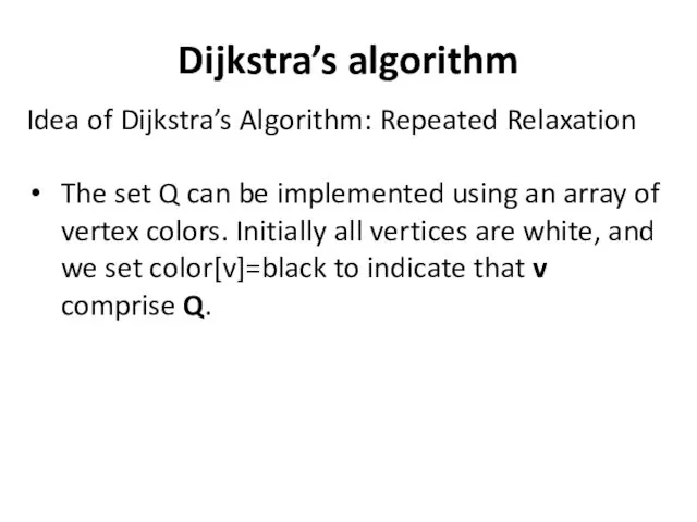
- 19. Dijkstra’s algorithm Idea of Dijkstra’s Algorithm: Repeated Relaxation The set Q can be implemented using an
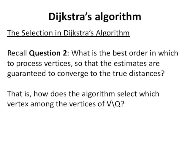
- 20. Dijkstra’s algorithm The Selection in Dijkstra’s Algorithm Recall Question 2: What is the best order in
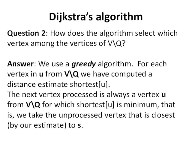
- 21. Dijkstra’s algorithm Question 2: How does the algorithm select which vertex among the vertices of V\Q?
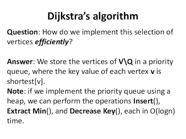
- 22. Dijkstra’s algorithm Question: How do we implement this selection of vertices efficiently? Answer: We store the
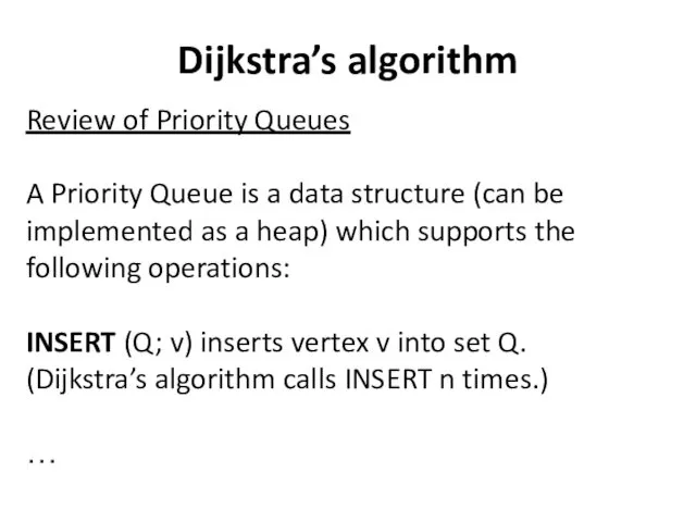
- 23. Dijkstra’s algorithm Review of Priority Queues A Priority Queue is a data structure (can be implemented
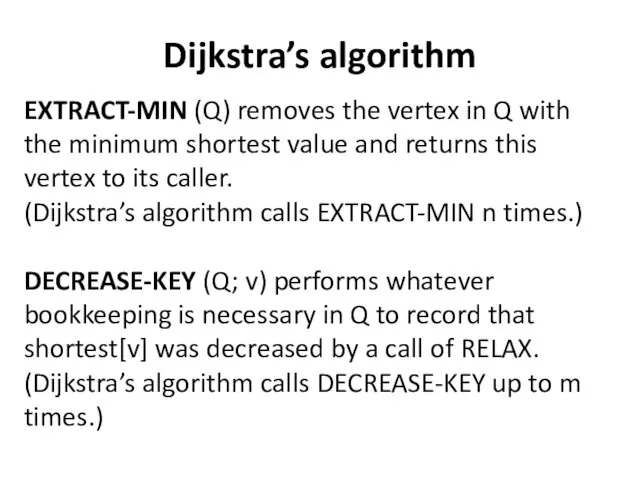
- 24. Dijkstra’s algorithm EXTRACT-MIN (Q) removes the vertex in Q with the minimum shortest value and returns
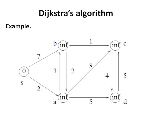
- 25. Dijkstra’s algorithm Example.
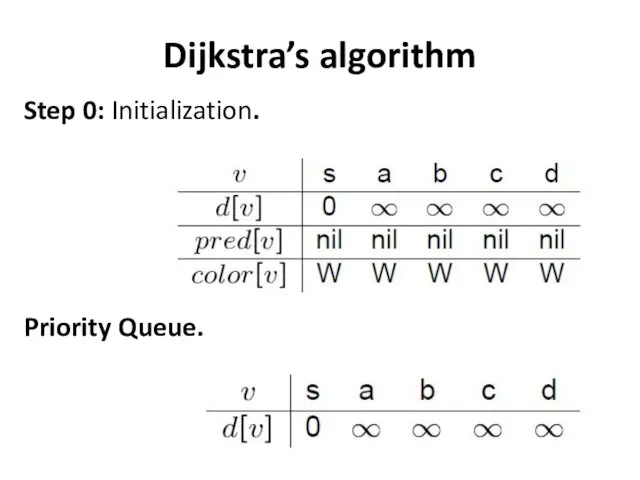
- 26. Dijkstra’s algorithm Step 0: Initialization. Priority Queue.
- 27. Dijkstra’s algorithm Step 1: As Adjacent[s]={a,b}, work on a and b and update information. Priority Queue:
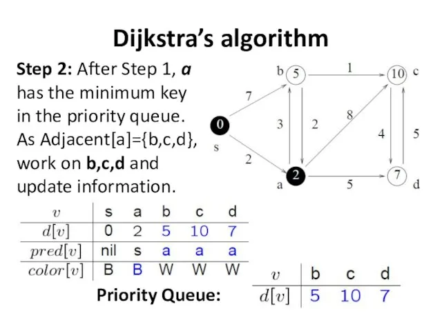
- 28. Dijkstra’s algorithm Step 2: After Step 1, a has the minimum key in the priority queue.
- 29. Dijkstra’s algorithm Step 3: After Step 2, b has the minimum key in the priority queue.
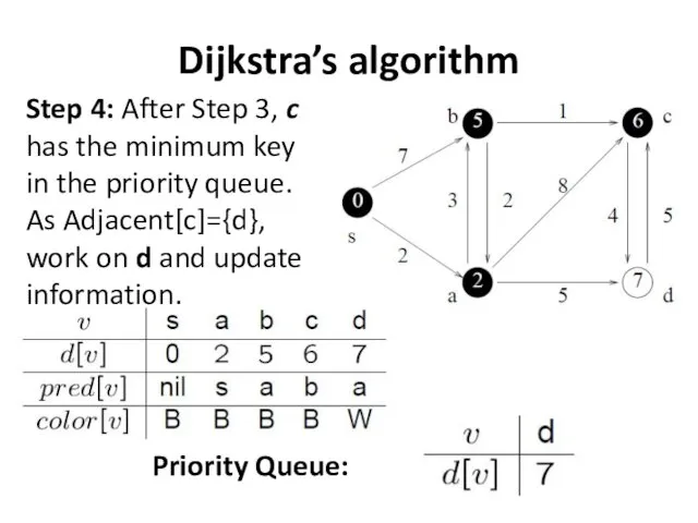
- 30. Dijkstra’s algorithm Step 4: After Step 3, c has the minimum key in the priority queue.
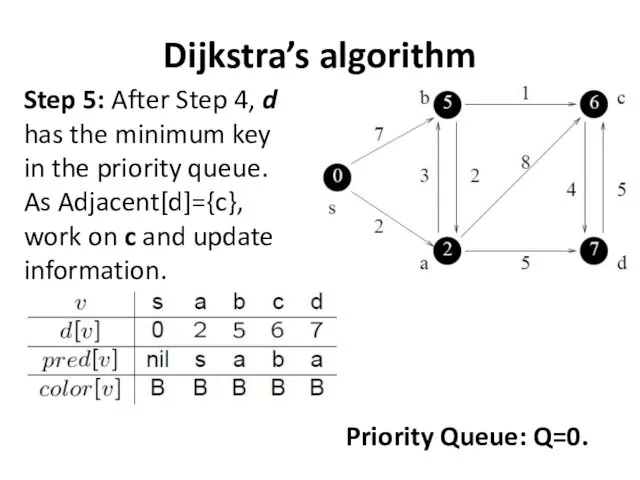
- 31. Dijkstra’s algorithm Step 5: After Step 4, d has the minimum key in the priority queue.
- 32. Dijkstra’s algorithm Shortest Path Tree: T=(V,A), where A={(pred[v],v)|v from V\{s}}. The array pred[v] is used to
- 33. Dijkstra’s algorithm
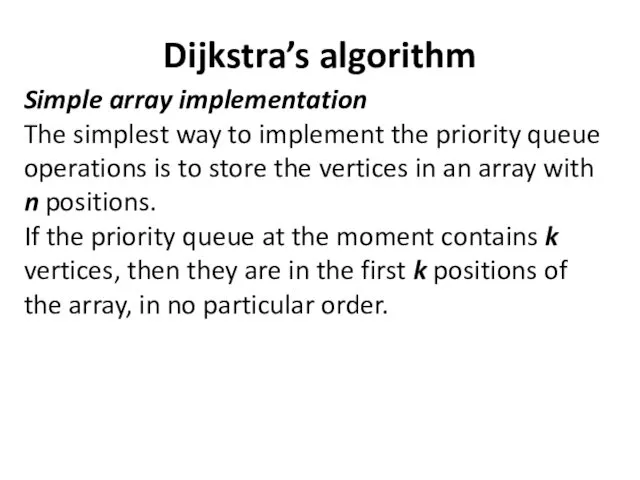
- 34. Dijkstra’s algorithm Simple array implementation The simplest way to implement the priority queue operations is to
- 35. Dijkstra’s algorithm Simple array implementation The INSERT operation is easy: just add the vertex to the
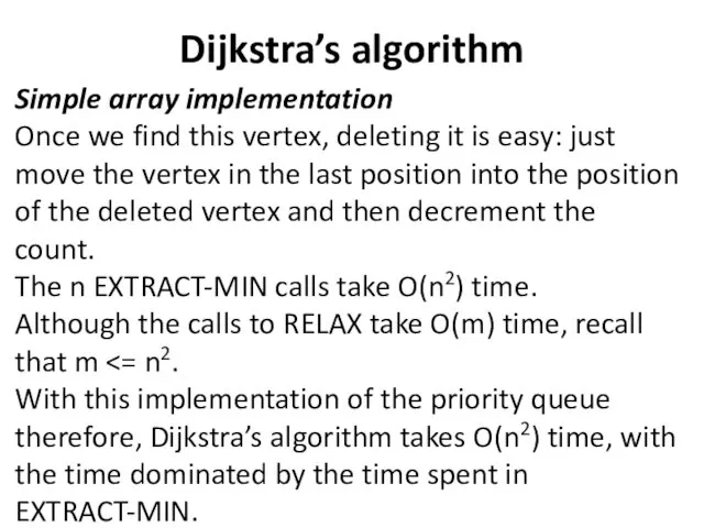
- 36. Dijkstra’s algorithm Simple array implementation Once we find this vertex, deleting it is easy: just move
- 37. Dijkstra’s algorithm Binary heap implementation A binary heap organizes data as a binary tree stored in
- 38. Dijkstra’s algorithm
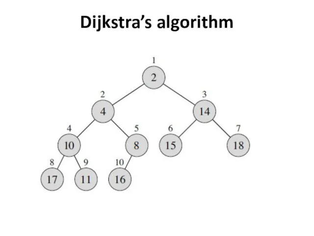
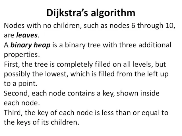
- 39. Dijkstra’s algorithm Nodes with no children, such as nodes 6 through 10, are leaves. A binary
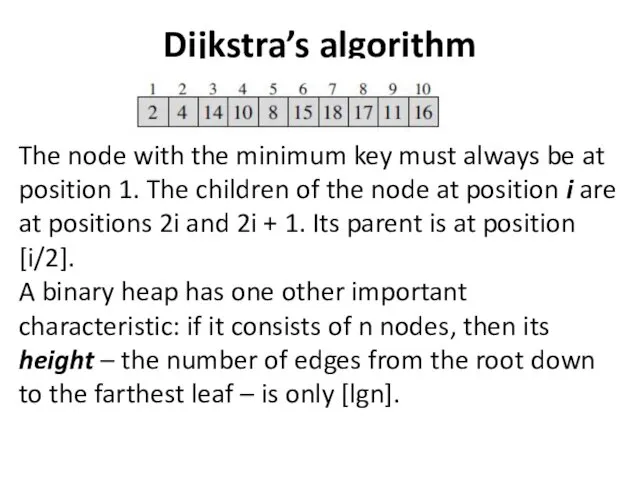
- 40. Dijkstra’s algorithm The node with the minimum key must always be at position 1. The children
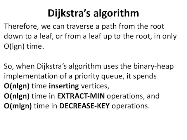
- 41. Dijkstra’s algorithm Therefore, we can traverse a path from the root down to a leaf, or
- 43. Скачать презентацию
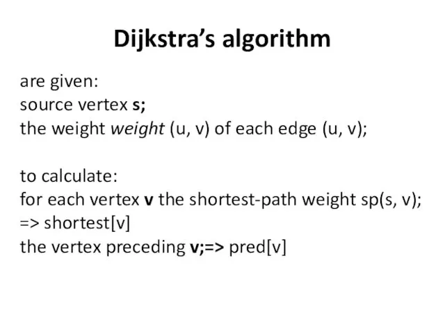
Dijkstra’s algorithm
are given:
source vertex s;
the weight weight (u, v) of each
Dijkstra’s algorithm
are given:
source vertex s;
the weight weight (u, v) of each
Dijkstra’s algorithm
Dijkstra’s algorithm
![Dijkstra’s algorithm the situation at time 0 shortest[s]= 0](/_ipx/f_webp&q_80&fit_contain&s_1440x1080/imagesDir/jpg/486175/slide-3.jpg)
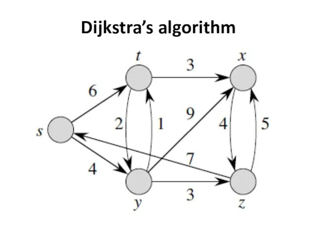
Dijkstra’s algorithm
the situation at time 0
shortest[s]= 0
Dijkstra’s algorithm
the situation at time 0
shortest[s]= 0
![Dijkstra’s algorithm at time 4 shortest[y]= 4, pred[y]= s](/_ipx/f_webp&q_80&fit_contain&s_1440x1080/imagesDir/jpg/486175/slide-4.jpg)
Dijkstra’s algorithm
at time 4
shortest[y]= 4, pred[y]= s
Dijkstra’s algorithm
at time 4
shortest[y]= 4, pred[y]= s
![Dijkstra’s algorithm at time 5 shortest[t]=5, pred[t]= y](/_ipx/f_webp&q_80&fit_contain&s_1440x1080/imagesDir/jpg/486175/slide-5.jpg)
Dijkstra’s algorithm
at time 5
shortest[t]=5, pred[t]= y
Dijkstra’s algorithm
at time 5
shortest[t]=5, pred[t]= y
![Dijkstra’s algorithm at time 7 shortest[z]=7, pred[z]= y](/_ipx/f_webp&q_80&fit_contain&s_1440x1080/imagesDir/jpg/486175/slide-6.jpg)
Dijkstra’s algorithm
at time 7
shortest[z]=7, pred[z]= y
Dijkstra’s algorithm
at time 7
shortest[z]=7, pred[z]= y
![Dijkstra’s algorithm at time 8 shortest[x]=8, pred[x]=t](/_ipx/f_webp&q_80&fit_contain&s_1440x1080/imagesDir/jpg/486175/slide-7.jpg)
Dijkstra’s algorithm
at time 8
shortest[x]=8, pred[x]=t
Dijkstra’s algorithm
at time 8
shortest[x]=8, pred[x]=t
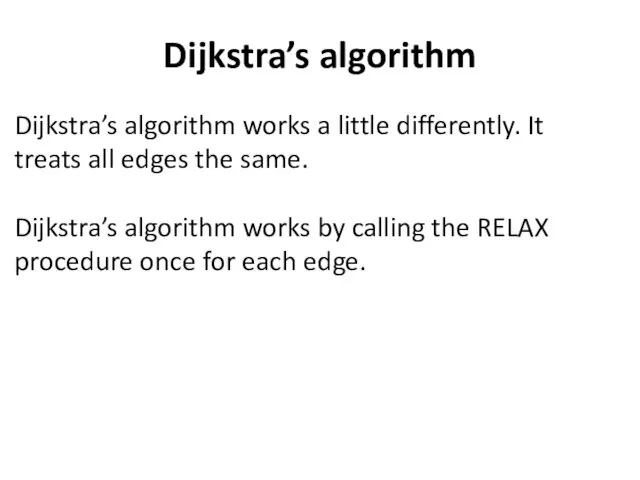
Dijkstra’s algorithm
Dijkstra’s algorithm works a little differently. It treats all edges
Dijkstra’s algorithm
Dijkstra’s algorithm works a little differently. It treats all edges

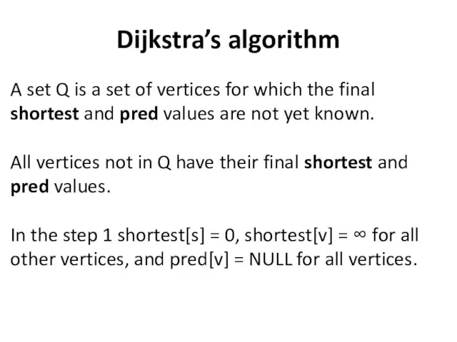
Dijkstra’s algorithm
A set Q is a set of vertices for which
Dijkstra’s algorithm
A set Q is a set of vertices for which
Dijkstra’s algorithm
A set Q is a set of vertices for which
Dijkstra’s algorithm
A set Q is a set of vertices for which
Dijkstra’s algorithm
Question 1: How does the algorithm find new paths and
Dijkstra’s algorithm
Question 1: How does the algorithm find new paths and
Dijkstra’s algorithm
Dijkstra’s algorithm
Dijkstra’s algorithm
Answer to Question 1: How does the algorithm find new
Dijkstra’s algorithm
Answer to Question 1: How does the algorithm find new
Dijkstra’s algorithm
Remaid: The Algorithm for Relaxing an Edge.
Relax(u, v)
{
If (shortest[u] +
Dijkstra’s algorithm
Remaid: The Algorithm for Relaxing an Edge.
Relax(u, v)
{
If (shortest[u] +
Dijkstra’s algorithm
Idea of Dijkstra’s Algorithm: Repeated Relaxation
Dijkstra’s algorithm operates by maintaining
Dijkstra’s algorithm
Idea of Dijkstra’s Algorithm: Repeated Relaxation
Dijkstra’s algorithm operates by maintaining
Dijkstra’s algorithm
Idea of Dijkstra’s Algorithm: Repeated Relaxation
Initially Q=NULL, the empty set,
Dijkstra’s algorithm
Idea of Dijkstra’s Algorithm: Repeated Relaxation
Initially Q=NULL, the empty set,
Dijkstra’s algorithm
Idea of Dijkstra’s Algorithm: Repeated Relaxation
The set Q can be
Dijkstra’s algorithm
Idea of Dijkstra’s Algorithm: Repeated Relaxation
The set Q can be
Dijkstra’s algorithm
The Selection in Dijkstra’s Algorithm
Recall Question 2: What is the
Dijkstra’s algorithm
The Selection in Dijkstra’s Algorithm
Recall Question 2: What is the
Dijkstra’s algorithm
Question 2: How does the algorithm select which vertex among
Dijkstra’s algorithm
Question 2: How does the algorithm select which vertex among
Dijkstra’s algorithm
Question: How do we implement this selection of vertices efficiently?
Answer:
Dijkstra’s algorithm
Question: How do we implement this selection of vertices efficiently?
Answer:
Dijkstra’s algorithm
Review of Priority Queues
A Priority Queue is a data structure
Dijkstra’s algorithm
Review of Priority Queues
A Priority Queue is a data structure
Dijkstra’s algorithm
EXTRACT-MIN (Q) removes the vertex in Q with the minimum
Dijkstra’s algorithm
EXTRACT-MIN (Q) removes the vertex in Q with the minimum
Dijkstra’s algorithm
Example.
Dijkstra’s algorithm
Example.
Dijkstra’s algorithm
Step 0: Initialization.
Priority Queue.
Dijkstra’s algorithm
Step 0: Initialization.
Priority Queue.
![Dijkstra’s algorithm Step 1: As Adjacent[s]={a,b}, work on a and b and update information. Priority Queue:](/_ipx/f_webp&q_80&fit_contain&s_1440x1080/imagesDir/jpg/486175/slide-26.jpg)
Dijkstra’s algorithm
Step 1: As Adjacent[s]={a,b},
work on a and b and update
Dijkstra’s algorithm
Step 1: As Adjacent[s]={a,b},
work on a and b and update
Dijkstra’s algorithm
Step 2: After Step 1, a has the minimum key
Dijkstra’s algorithm
Step 2: After Step 1, a has the minimum key

Dijkstra’s algorithm
Step 3: After Step 2, b has the minimum key
Dijkstra’s algorithm
Step 3: After Step 2, b has the minimum key
Dijkstra’s algorithm
Step 4: After Step 3, c has the minimum key
Dijkstra’s algorithm
Step 4: After Step 3, c has the minimum key
Dijkstra’s algorithm
Step 5: After Step 4, d has the minimum key
Dijkstra’s algorithm
Step 5: After Step 4, d has the minimum key
![Dijkstra’s algorithm Shortest Path Tree: T=(V,A), where A={(pred[v],v)|v from V\{s}}. The](/_ipx/f_webp&q_80&fit_contain&s_1440x1080/imagesDir/jpg/486175/slide-31.jpg)
Dijkstra’s algorithm
Shortest Path Tree: T=(V,A),
where A={(pred[v],v)|v from V\{s}}.
The array pred[v]
Dijkstra’s algorithm
Shortest Path Tree: T=(V,A),
where A={(pred[v],v)|v from V\{s}}.
The array pred[v]
Dijkstra’s algorithm
Dijkstra’s algorithm
Dijkstra’s algorithm
Simple array implementation
The simplest way to implement the priority queue
Dijkstra’s algorithm
Simple array implementation
The simplest way to implement the priority queue

Dijkstra’s algorithm
Simple array implementation
The INSERT operation is easy: just add the
Dijkstra’s algorithm
Simple array implementation
The INSERT operation is easy: just add the
Dijkstra’s algorithm
Simple array implementation
Once we find this vertex, deleting it is
Dijkstra’s algorithm
Simple array implementation
Once we find this vertex, deleting it is

Dijkstra’s algorithm
Binary heap implementation
A binary heap organizes data as a binary
Dijkstra’s algorithm
Binary heap implementation
A binary heap organizes data as a binary
Dijkstra’s algorithm
Dijkstra’s algorithm
Dijkstra’s algorithm
Nodes with no children, such as nodes 6 through 10,
Dijkstra’s algorithm
Nodes with no children, such as nodes 6 through 10,
Dijkstra’s algorithm
The node with the minimum key must always be at
Dijkstra’s algorithm
The node with the minimum key must always be at
Dijkstra’s algorithm
Therefore, we can traverse a path from the root down
Dijkstra’s algorithm
Therefore, we can traverse a path from the root down
 Аттестационная работа. Рабочая программа математического кружка в 5 классе: Математика плюс
 Постороение сечений
 КАК ГОТОВИТЬСЯ к ГИА-9 по математике Учитель математики Воронина Т.К.
  Задачи на железнодорожную тему
 Презентация по математике "Теорема косинусов в электронных таблицах" - скачать
  Теорема Пифагора
 Статистика знает всё
 Алгоритм решения квадратных неравенств
 Площадь круга
 Тема: « Задачи на построение сечений».
  Призма
 Пирамида в задачах ЕГЭ
 Паркеты из многоугольников
 Касательная. Уравнение касательной
 Вводное повторение.Геометрия 8 класс
 Туынды. Алғашқы функция. Интеграл
 Замечательный квадрат. Урок по математике в 5 классе
 Геометрия. 7 класс
 Фунцияның туындысы мен дифференциалын қолдану
 Линейные дискретные системы. Описание ЛДС во временной области
 Общая математическая модель динамики
 Подготовка к ГИА по математике. Задания 13
 Как записывают и читают десятичные дроби
 Решение неравенств
 Объемы тел
 Изучение взаимосвязи между явлениями методами корреляционно-регрессионного анализа
 Геометрические иллюзии, или всегда ли мы видим то, что видим
 Что такое процент