- The mean values

Содержание
- 2. Part 1 THE MEAN VALUES
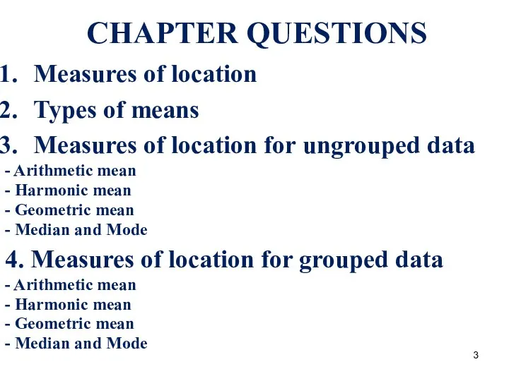
- 3. СHAPTER QUESTIONS Measures of location Types of means Measures of location for ungrouped data - Arithmetic
- 4. Properties to describe numerical data: Central tendency Dispersion Shape Measures calculated for: Sample data Statistics Entire
- 5. Measures of location include: Arithmetic mean Harmonic mean Geometric mean Median Mode Measures of location and
- 6. Grouped and Ungrouped UNGROUPED or raw data refers to data as they were collected, that is,
- 7. What is the mean? The mean - is a general indicator characterizing the typical level of
- 8. Statistics derive the formula of the means of the formula of mean exponential: We introduce the
- 9. There are the following types of mean: If z = -1 - the harmonic mean, z
- 10. The higher the degree of z, the greater the value of the mean. If the characteristic
- 11. There are two ways of calculating mean: for ungrouped data - is calculated as a simple
- 12. Types of means
- 13. Arithmetic mean Arithmetic mean value is called the mean value of the sign, in the calculation
- 14. Characteristics of the arithmetic mean The arithmetic mean has a number of mathematical properties that can
- 15. 2. If the data values (Xi) divided or multiplied by a constant number (A), the mean
- 16. 3. If the frequency divided by a constant number, the mean will not change:
- 17. 4. Multiplying the mean for the amount of frequency equal to the sum of multiplications variants
- 18. 5.The sum of the deviations of the number in a data value from the mean is
- 19. Measures of location for ungrouped data In calculating summary values for a data collection, the best
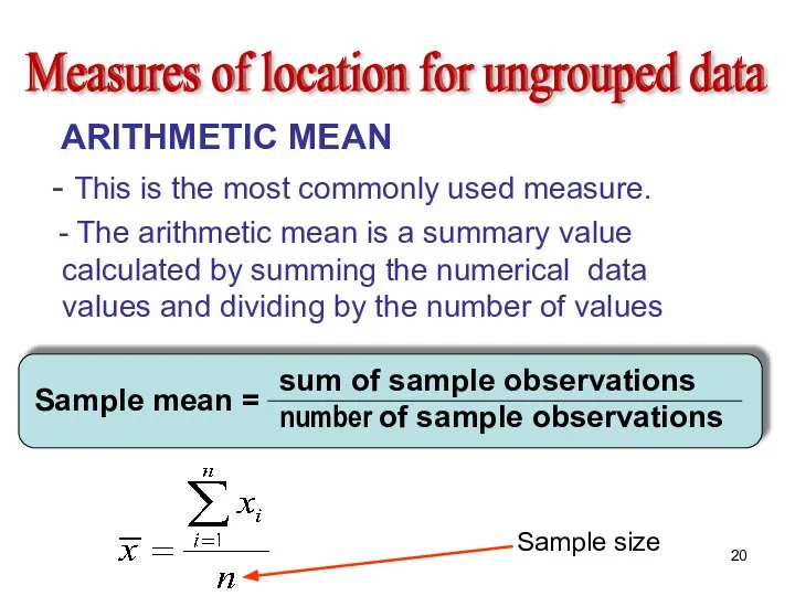
- 20. Measures of location for ungrouped data ARITHMETIC MEAN - This is the most commonly used measure.
- 21. sum of observations number of observations Population mean = Measures of location for ungrouped data ARITHMETIC
- 22. Example - The sales of the six largest restaurant chains are presented in table A mean
- 23. MEDIAN for ungrouped data The median of a data is the middle item in a set
- 24. MEDIAN Every ordinal-level, interval-level and ratio-level data set has a median The median is not sensitive
- 25. Position of median If n is odd: Median item number = (n+1)/2 If n is even:
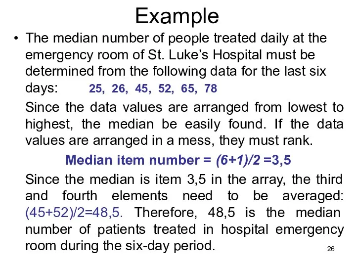
- 26. Example The median number of people treated daily at the emergency room of St. Luke’s Hospital
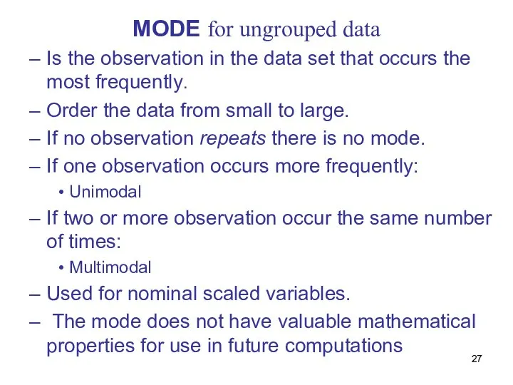
- 27. MODE for ungrouped data Is the observation in the data set that occurs the most frequently.
- 28. The simple mean of the sample of nine measurements is given by: 2 5 8 5
- 29. −4 −3 2 2 5 5 5 6 8 Median item number = (n+1)/2 = (9+1)/2
- 30. Determine the median of the sample of ten measurements. Order the measurements Example Given the following
- 31. Determine the mode of the sample of nine measurements. Order the measurements Given the following data
- 32. Determine the mode of the sample of ten measurements. Order the measurements Given the following data
- 33. Is used if М = const: Harmonic mean is also called the simple mean of the
- 34. For example: One student spends on a solution of task 1/3 hours, the second student –
- 35. Geometric mean for ungrouped data This value is used as the average of the relations between
- 36. Where П – the multiplication of the data value (Xi). n – power of root Geometric
- 37. For example, the known data about the rate of growth of production Calculate the geometric mean.
- 38. Measures of location for grouped data ARITHMETIC MEAN Data is given in a frequency table Only
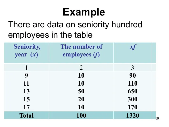
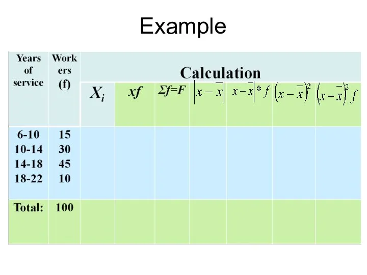
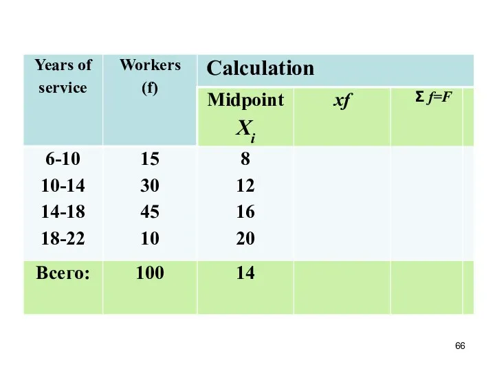
- 39. Example There are data on seniority hundred employees in the table
- 40. Average seniority employee is:
- 41. Harmonic mean for grouped data Harmonic mean - is the reciprocal of the arithmetic mean. Harmonic
- 42. Harmonic mean for grouped data Harmonic mean is calculated by the formula: where M = xf
- 43. Example There are data on hárvesting the apples by three teams and on average per worker
- 44. is calculated by the formula: Where fi – frequency of the data value (Xi) П –
- 45. Calculate the geometric mean. It is 127,5% percent: Geometric mean for grouped data EXAMPLE
- 46. Measures of location for grouped data MEDIAN Data is given in a frequency table. First cumulative
- 47. Measures of location for grouped data MODE Class interval that has the largest frequency value will
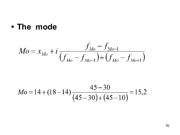
- 48. Mode is calculated by the formula: where хМо – lower boundary of the modal interval i=
- 49. To calculate the mean for the sample of the 48 hours: Determine the class midpoints Number
- 50. Number of Number of xi calls hours fi [2–under 5) 3 3,5 [5–under 8) 4 6,5
- 51. To calculate the for the sample median of the 48: hours: determine the cumulative frequencies Number
- 52. Number of Number of calls hours fi F [2–under 5) 3 3 [5–under 8) 4 7
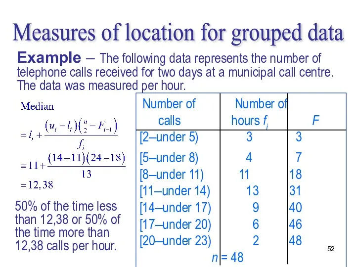
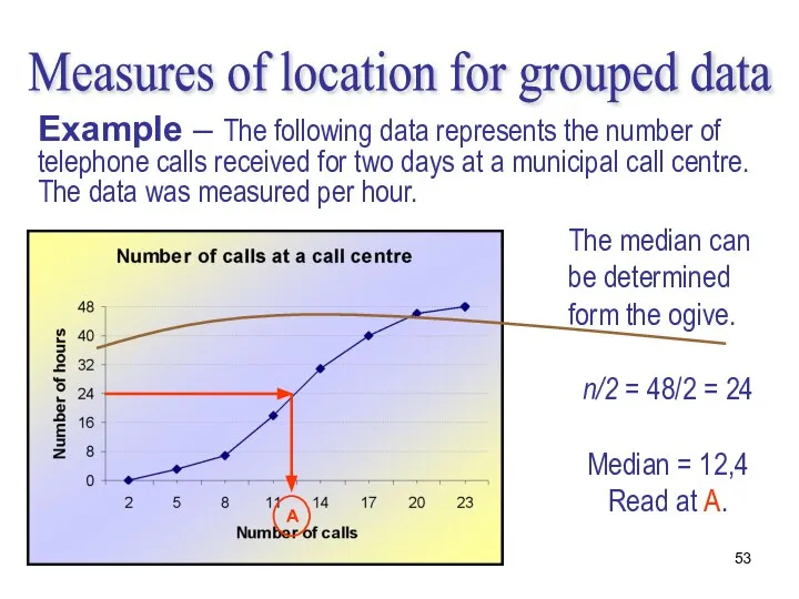
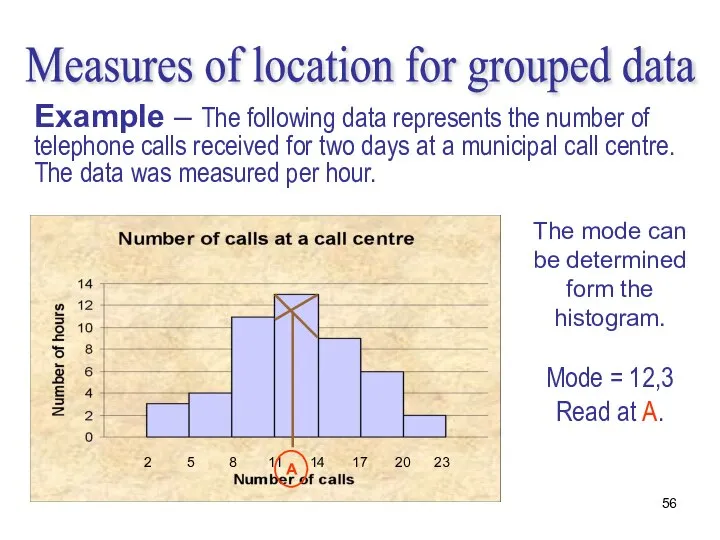
- 53. Measures of location for grouped data Example – The following data represents the number of telephone
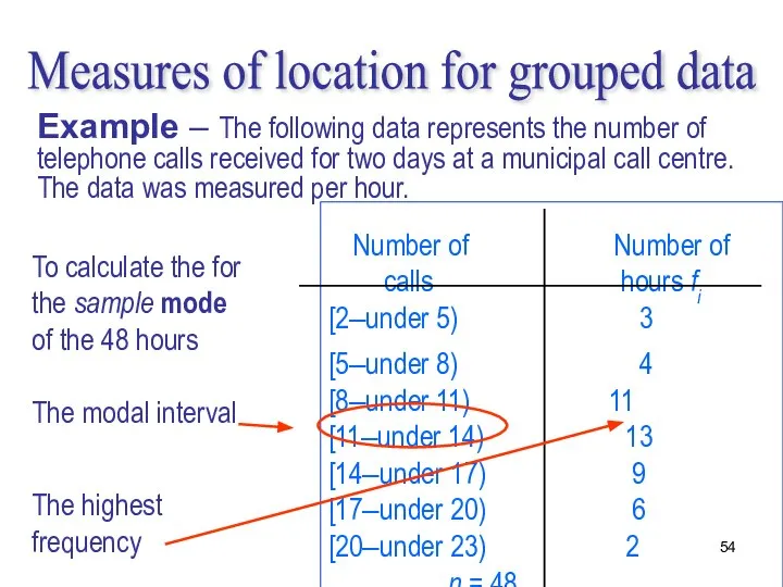
- 54. To calculate the for the sample mode of the 48 hours The modal interval Number of
- 55. We substitute the data into the formula: Mo = 12,3 So, the most frequent number of
- 56. Measures of location for grouped data Example – The following data represents the number of telephone
- 57. Relationship between mean, median, and mode If a distribution is symmetrical: the mean, median and mode
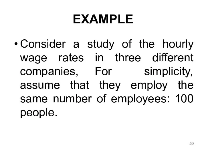
- 59. EXAMPLE Consider a study of the hourly wage rates in three different companies, For simplicity, assume
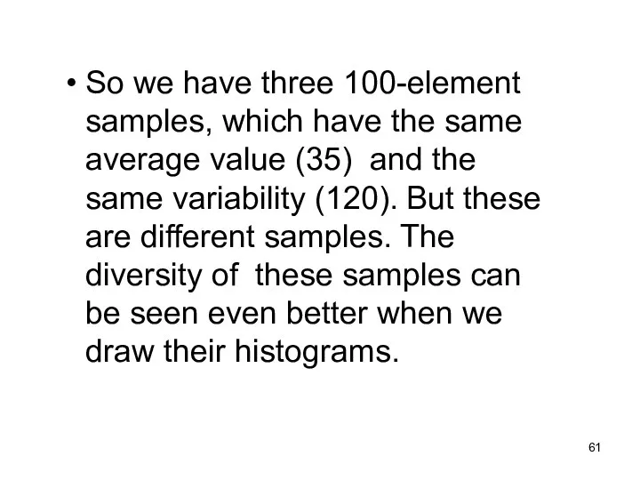
- 61. So we have three 100-element samples, which have the same average value (35) and the same
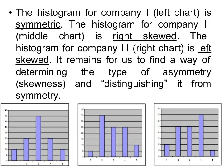
- 62. The histogram for company I (left chart) is symmetric. The histogram for company II (middle chart)
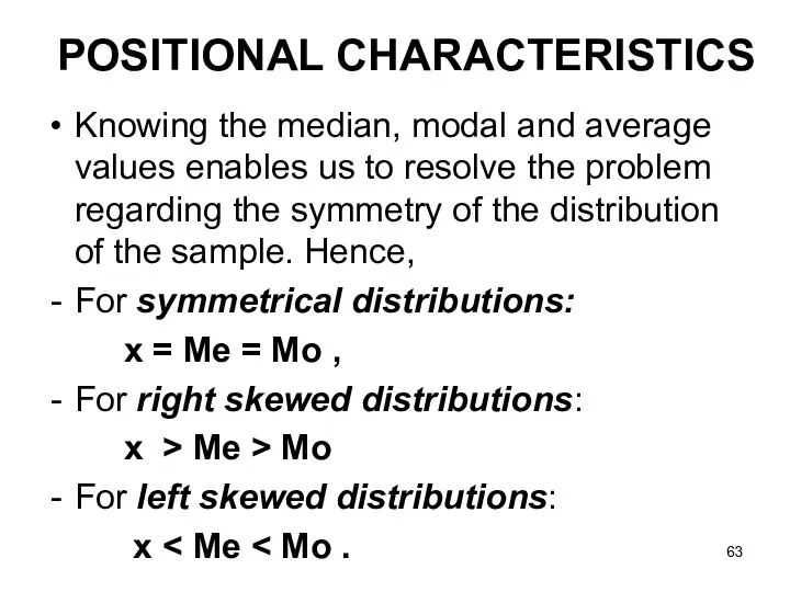
- 63. Knowing the median, modal and average values enables us to resolve the problem regarding the symmetry
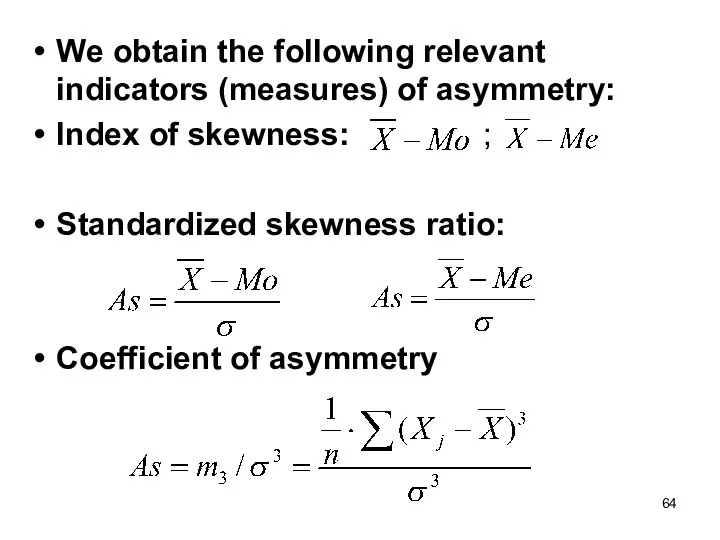
- 64. We obtain the following relevant indicators (measures) of asymmetry: Index of skewness: ; Standardized skewness ratio:
- 65. Example
- 68. The weighted arithmetic mean
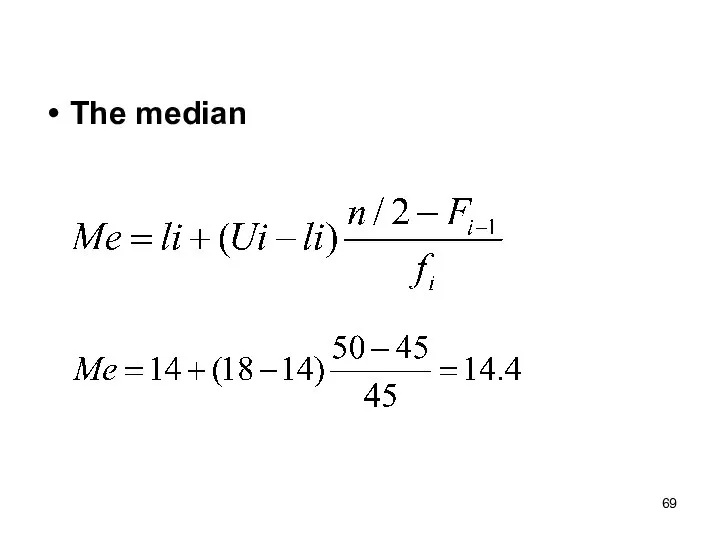
- 69. The median
- 70. The mode
- 72. Скачать презентацию
Part 1
THE MEAN VALUES
Part 1
THE MEAN VALUES
СHAPTER QUESTIONS
Measures of location
Types of means
Measures of location for ungrouped data
-
СHAPTER QUESTIONS
Measures of location
Types of means
Measures of location for ungrouped data
-
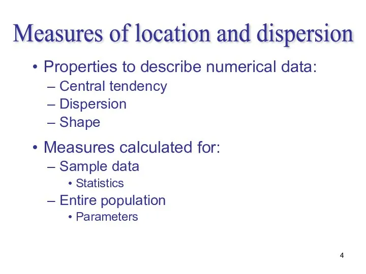
Properties to describe numerical data:
Central tendency
Dispersion
Shape
Measures calculated for:
Sample data
Statistics
Entire population
Parameters
Measures of
Properties to describe numerical data:
Central tendency
Dispersion
Shape
Measures calculated for:
Sample data
Statistics
Entire population
Parameters
Measures of
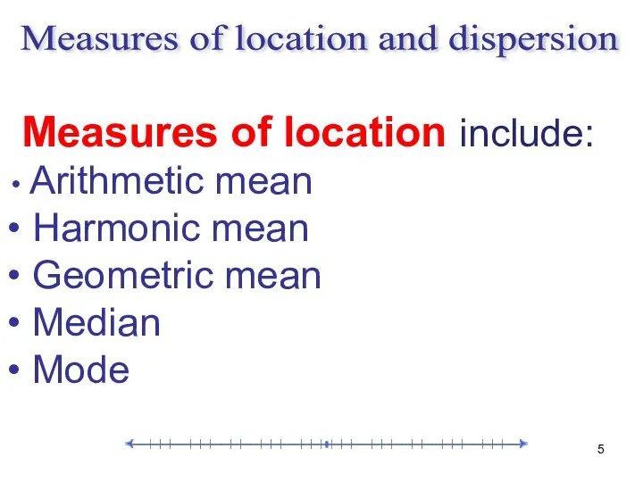
Measures of location include:
Arithmetic mean
Harmonic mean
Geometric mean
Median
Measures of location include:
Arithmetic mean
Harmonic mean
Geometric mean
Median
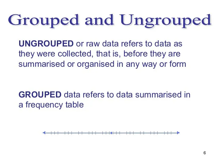
Grouped and Ungrouped
UNGROUPED or raw data refers to data as
Grouped and Ungrouped
UNGROUPED or raw data refers to data as
What is the mean?
The mean - is a general indicator characterizing
What is the mean?
The mean - is a general indicator characterizing
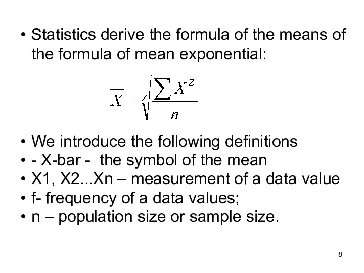
Statistics derive the formula of the means of the formula of
Statistics derive the formula of the means of the formula of
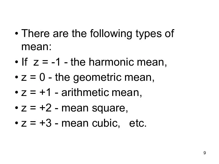
There are the following types of mean:
If z = -1
There are the following types of mean:
If z = -1
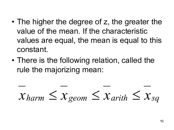
The higher the degree of z, the greater the value of
The higher the degree of z, the greater the value of
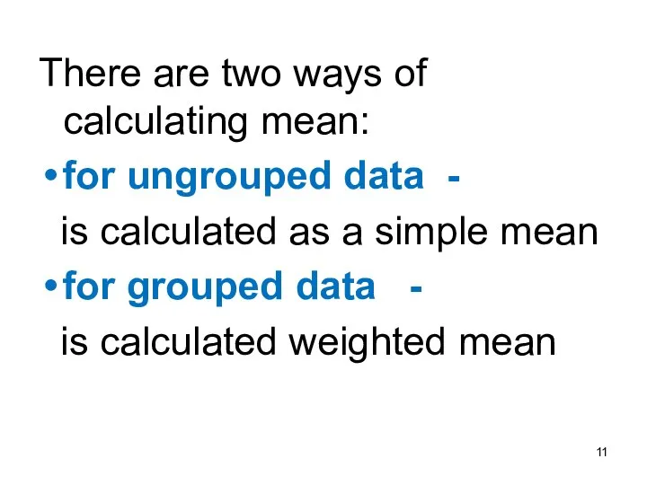
There are two ways of calculating mean:
for ungrouped data -
There are two ways of calculating mean:
for ungrouped data -
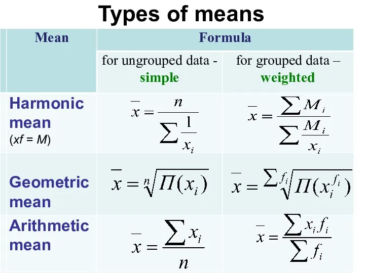
Types of means
Types of means
Arithmetic mean
Arithmetic mean value is called the mean value of
Arithmetic mean
Arithmetic mean value is called the mean value of
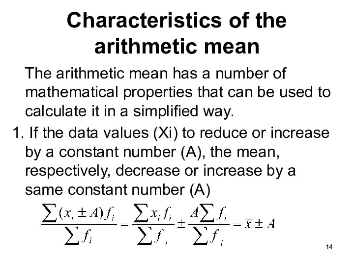
Characteristics of the arithmetic mean
The arithmetic mean has a number
Characteristics of the arithmetic mean
The arithmetic mean has a number
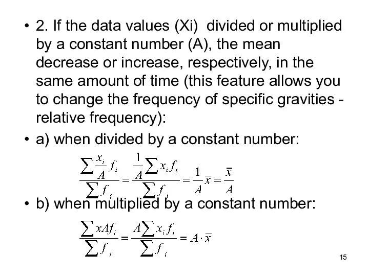
2. If the data values (Xi) divided or multiplied by a
2. If the data values (Xi) divided or multiplied by a
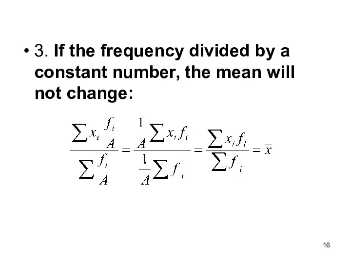
3. If the frequency divided by a constant number, the mean
3. If the frequency divided by a constant number, the mean
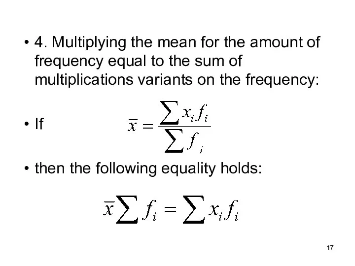
4. Multiplying the mean for the amount of frequency equal to
4. Multiplying the mean for the amount of frequency equal to
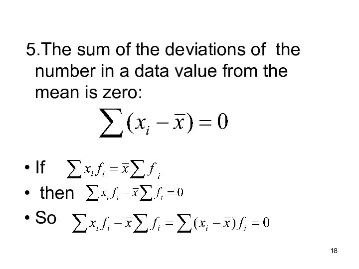
5.The sum of the deviations of the number in a
5.The sum of the deviations of the number in a
Measures of location for ungrouped data
In calculating summary values for a
Measures of location for ungrouped data
In calculating summary values for a
Measures of location for ungrouped data
ARITHMETIC MEAN
-
Measures of location for ungrouped data
ARITHMETIC MEAN
-
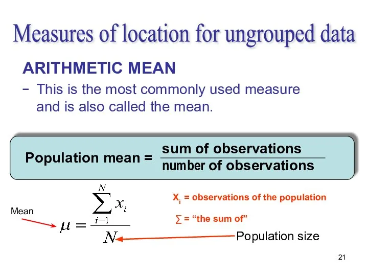
sum of observations
number of observations
Population mean =
Measures of location for
sum of observations
number of observations
Population mean =
Measures of location for
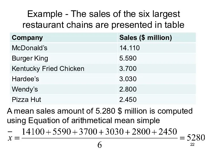
Example - The sales of the six largest restaurant chains are
Example - The sales of the six largest restaurant chains are
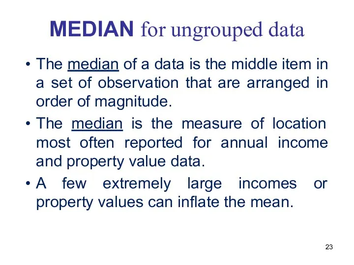
MEDIAN for ungrouped data
The median of a data is the middle
MEDIAN for ungrouped data
The median of a data is the middle
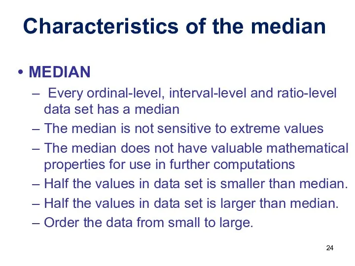
MEDIAN
Every ordinal-level, interval-level and ratio-level data set has a
MEDIAN
Every ordinal-level, interval-level and ratio-level data set has a
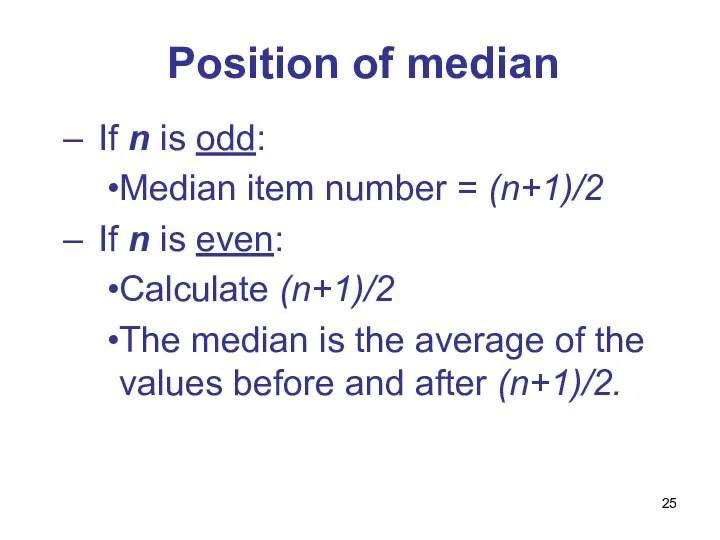
Position of median
If n is odd:
Median item number
Position of median
If n is odd:
Median item number
Example
The median number of people treated daily at the emergency
Example
The median number of people treated daily at the emergency
MODE for ungrouped data
Is the observation in the data set that
MODE for ungrouped data
Is the observation in the data set that
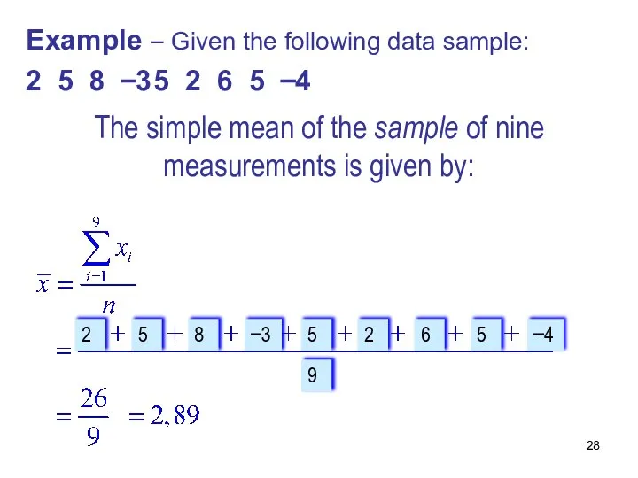
The simple mean of the sample of nine measurements is given
The simple mean of the sample of nine measurements is given
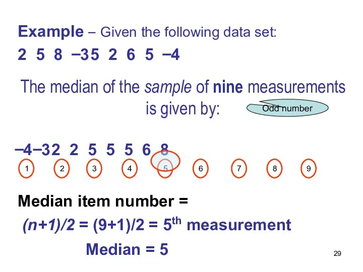
−4 −3 2 2 5 5 5 6 8
Median item number =
(n+1)/2 = (9+1)/2 = 5th measurement
1
2
3
4
5
6
7
8
9
Median =
−4 −3 2 2 5 5 5 6 8
Median item number =
(n+1)/2 = (9+1)/2 = 5th measurement
1
2
3
4
5
6
7
8
9
Median =
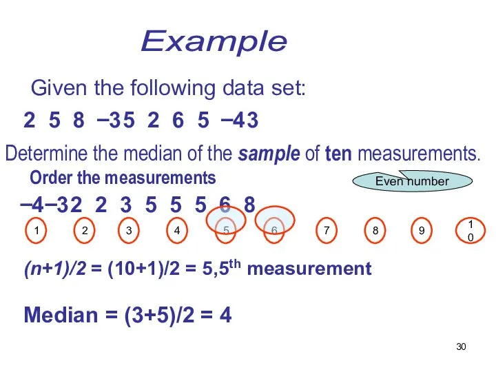
Determine the median of the sample of ten measurements.
Order the measurements
Example
Determine the median of the sample of ten measurements.
Order the measurements
Example
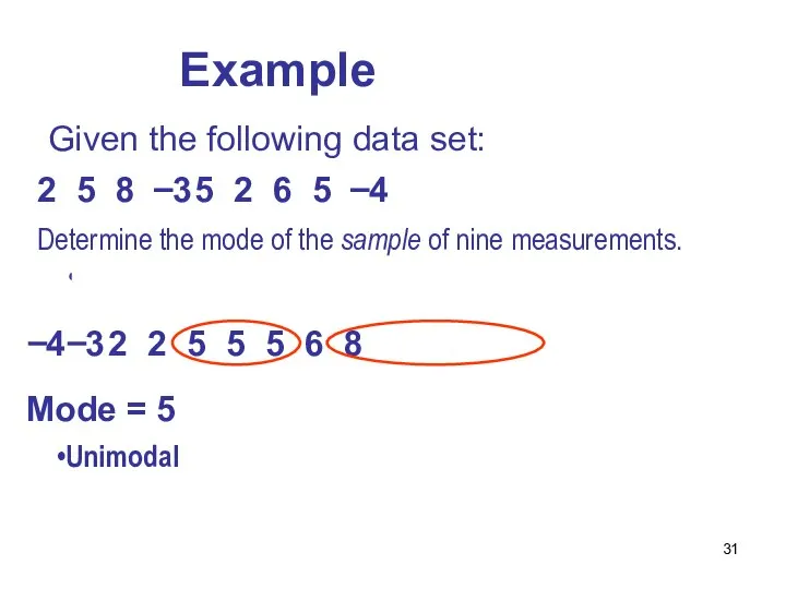
Determine the mode of the sample of nine measurements.
Order the measurements
Determine the mode of the sample of nine measurements.
Order the measurements
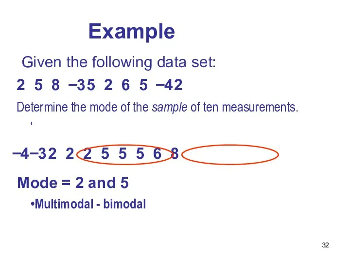
Determine the mode of the sample of ten measurements.
Order the measurements
Determine the mode of the sample of ten measurements.
Order the measurements
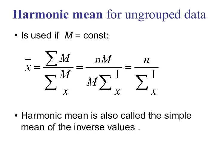
Is used if М = const:
Harmonic mean is also called the
Is used if М = const:
Harmonic mean is also called the
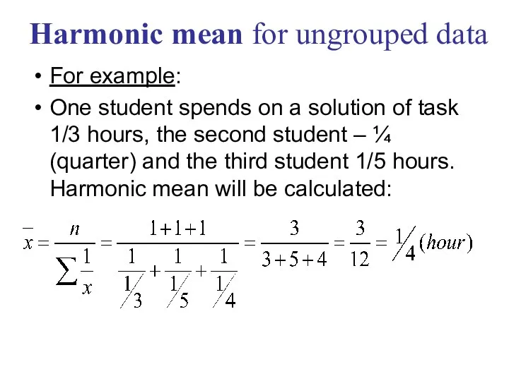
For example:
One student spends on a solution of task 1/3
One student spends on a solution of task 1/3
Geometric mean for ungrouped data
This value is used as the average
Geometric mean for ungrouped data
This value is used as the average
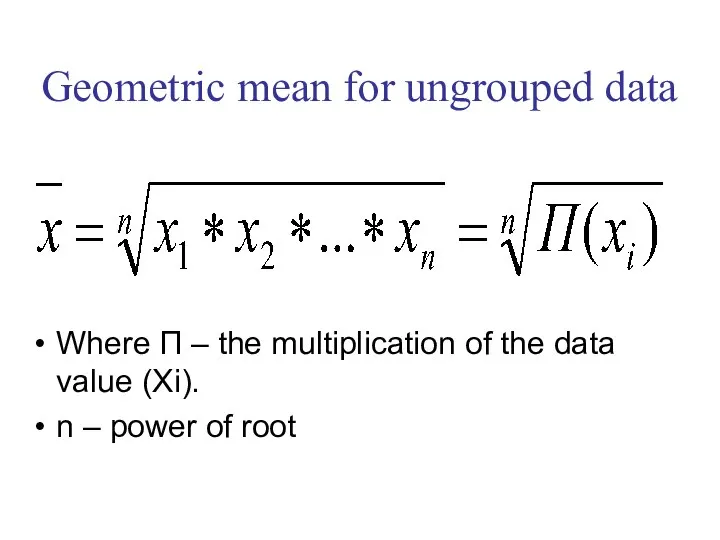
Where П – the multiplication of the data value (Xi).
n
Where П – the multiplication of the data value (Xi).
n
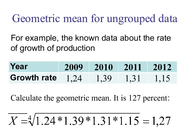
For example, the known data about the rate of growth of
For example, the known data about the rate of growth of
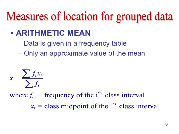
Measures of location for grouped data
ARITHMETIC MEAN
Data is given
Measures of location for grouped data
ARITHMETIC MEAN
Data is given
Example
There are data on seniority hundred employees in the table
Example
There are data on seniority hundred employees in the table
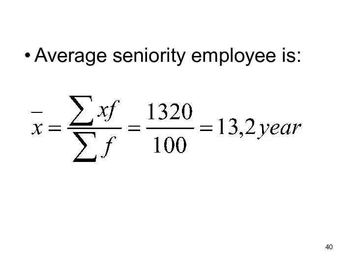
Average seniority employee is:
Average seniority employee is:

Harmonic mean for grouped data
Harmonic mean - is the reciprocal of
Harmonic mean for grouped data
Harmonic mean - is the reciprocal of
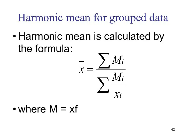
Harmonic mean for grouped data
Harmonic mean is calculated by the formula:
where
Harmonic mean for grouped data
Harmonic mean is calculated by the formula:
where
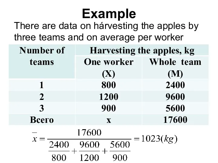
Example
There are data on hárvesting the apples by three teams
Example
There are data on hárvesting the apples by three teams
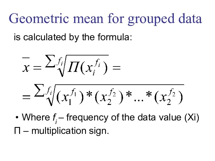
is calculated by the formula:
Where fi – frequency of the data
is calculated by the formula:
Where fi – frequency of the data
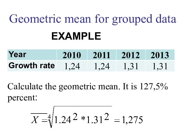
Calculate the geometric mean. It is 127,5% percent:
Geometric mean for grouped
Calculate the geometric mean. It is 127,5% percent:
Geometric mean for grouped
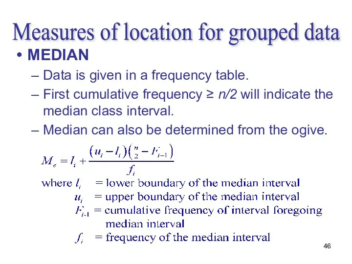
Measures of location for grouped data
MEDIAN
Data is given in
Measures of location for grouped data
MEDIAN
Data is given in
Measures of location for grouped data
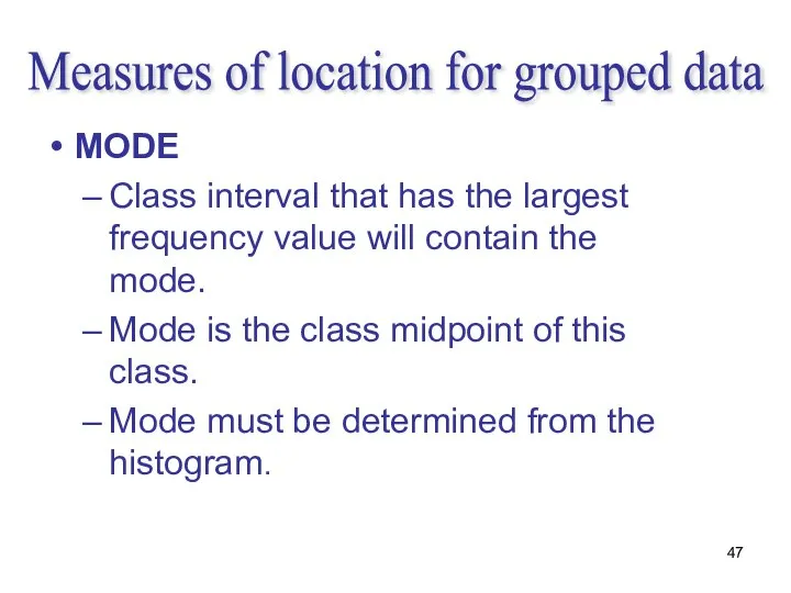
MODE
Class interval that has the
Measures of location for grouped data
MODE
Class interval that has the
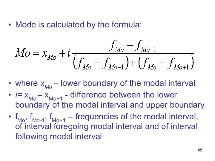
Mode is calculated by the formula:
where хМо – lower boundary of
Mode is calculated by the formula:
where хМо – lower boundary of
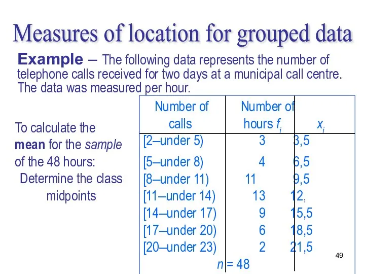
To calculate the mean for the sample of the 48 hours:
Determine
To calculate the mean for the sample of the 48 hours:
Determine
Number of Number of xi
calls hours fi
[2–under 5) 3 3,5
Number of Number of xi
calls hours fi
[2–under 5) 3 3,5
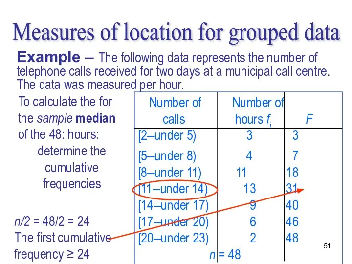
To calculate the for the sample median of the 48: hours:
determine
To calculate the for the sample median of the 48: hours:
determine
Number of Number of
calls hours fi F
[2–under 5)
Number of Number of
calls hours fi F
[2–under 5)
Measures of location for grouped data
Example – The following data
Measures of location for grouped data
Example – The following data
To calculate the for the sample mode of the 48 hours
The
To calculate the for the sample mode of the 48 hours
The
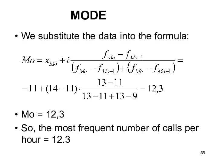
We substitute the data into the formula:
Mo = 12,3
So, the most
We substitute the data into the formula:
Mo = 12,3
So, the most
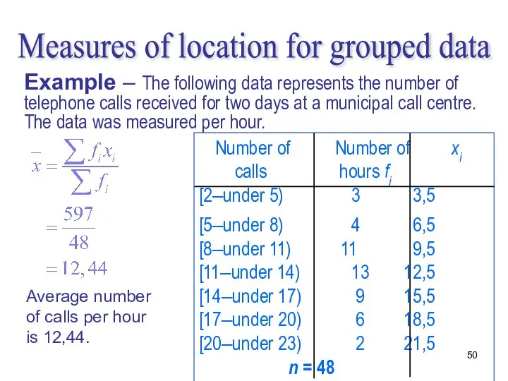
Measures of location for grouped data
Example – The following data
Measures of location for grouped data
Example – The following data

Relationship between mean, median, and mode
If a distribution is symmetrical:
the mean,
Relationship between mean, median, and mode
If a distribution is symmetrical:
the mean,

EXAMPLE
Consider a study of the hourly wage rates in three different
EXAMPLE
Consider a study of the hourly wage rates in three different
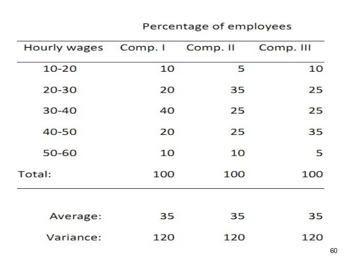
So we have three 100-element samples, which have the same average
So we have three 100-element samples, which have the same average
The histogram for company I (left chart) is symmetric. The histogram
The histogram for company I (left chart) is symmetric. The histogram
Knowing the median, modal and average values enables us to resolve
Knowing the median, modal and average values enables us to resolve
We obtain the following relevant indicators (measures) of asymmetry:
Index of
We obtain the following relevant indicators (measures) of asymmetry:
Index of
Example
Example

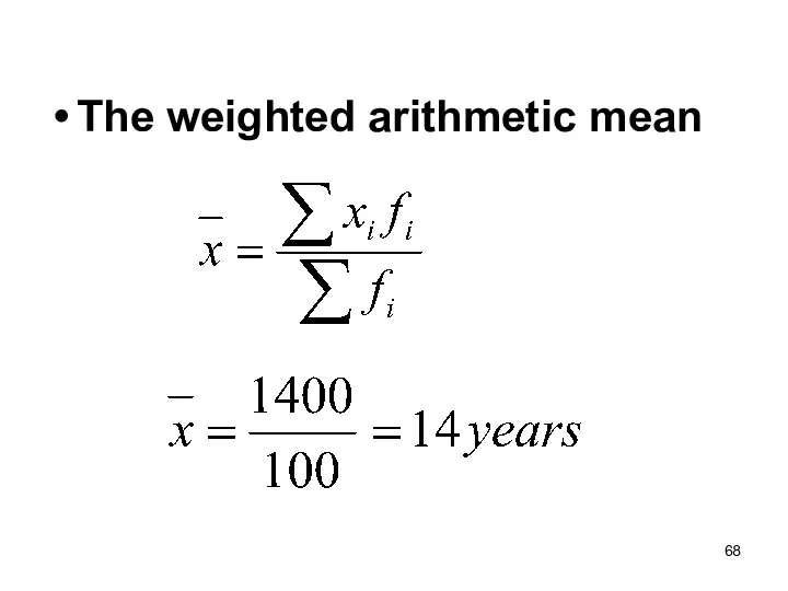
The weighted arithmetic mean
The weighted arithmetic mean
 Неравенство треугольника
 Решение заданий В9. Тригонометрия. Задания открытого банка задач
 Заседание клуба «Знатоков» Тема: Применение квадратных уравнений для решения задач. Тип урока: Повторение и обобщение знаний.
  Умножение и деление положительных и отрицательных чисел. Урок 48
 Среднее арифметическое. Математический диктант
 Шифры и математика
 Вписанная окружность
 Конструкция многообразий, ассоциированных с классическими системами корней
 Скалярное произведение векторов
 Софья Васильевна Ковалевская Работу выполнили: Ученицы 5 б класса Соловьева Арина и Уланова Ксения
 Предел функции
 Сложение и вычитание десятичных дробей ( 5 класс, математика)
 Практическое применение теорем геометрии в жизни
 Метод ветвей и границ. Решение задачи о коммивояжере
 Аттестационная работа. Исследовательская деятельность на уроках математики
 Теория множеств. (Лекция 5)
 Смежные и вертикальные углы
 Выборочное наблюдение
 Старинные единицы измерения
 Аттестационная работа. Длина и ее измерение
 Задачи на концентрацию, смеси и сплавы. Подготовка к ГИА
 Презентация по математике "Вычисления с многозначными числами" - скачать бесплатно
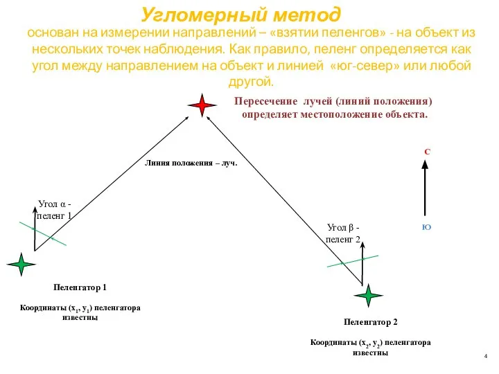 Угломерный метод
 Веселая математика
 Длина окружности. 6 класс
 тест по геометрии
 Длина окружности
 Параллельность прямых