- Data Structures and Algorithms

Содержание
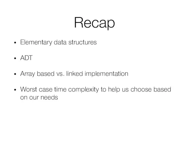
- 2. Recap Elementary data structures ADT Array based vs. linked implementation Worst case time complexity to help
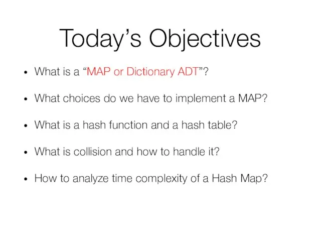
- 3. Today’s Objectives What is a “MAP or Dictionary ADT”? What choices do we have to implement
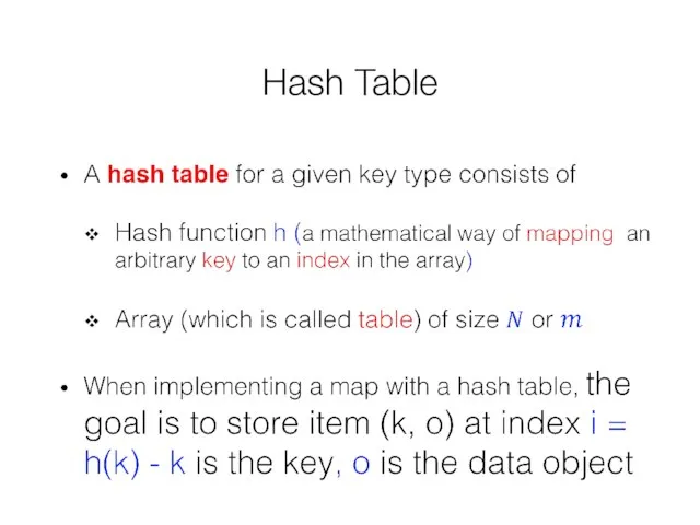
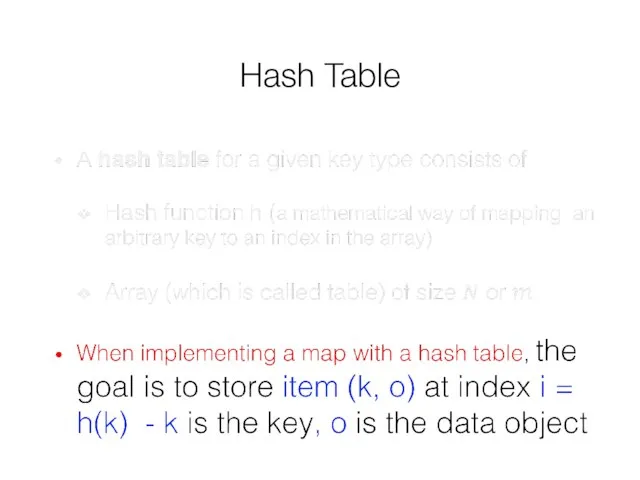
- 4. Map or Dictionary
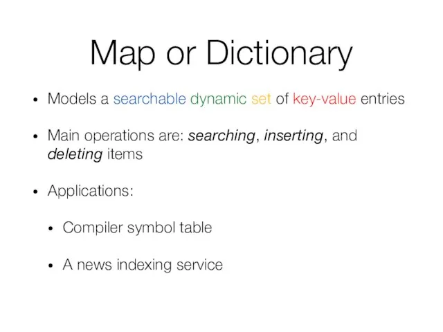
- 5. Map or Dictionary Models a searchable dynamic set of key-value entries Main operations are: searching, inserting,
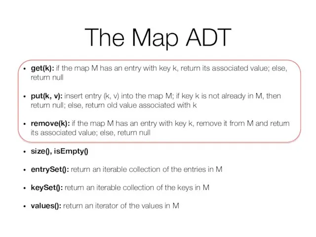
- 6. The Map ADT get(k): if the map M has an entry with key k, return its
- 7. Example Operation Output Map isEmpty() true Ø put(5,A) null (5,A) put(7,B) null (5,A),(7,B) put(2,C) null (5,A),(7,B),(2,C)
- 8. A Simple List-Based Map We can implement a map using an unsorted list We store the
- 9. The get(k) Algorithm Algorithm get(k): while map.hasNext() do p = map.next() { the next element in
- 10. The put(k,v) Algorithm Algorithm put(k,v): while map.hasNext() do p = map.next() if p.element().getKey() = k then
- 11. The remove(k) Algorithm Algorithm remove(k): while map.hasNext() do p = map.next() if p.element().getKey() = k then
- 12. Performance of a List-Based Map Performance: put takes O(1) time since we can insert the new
- 13. Hash Map
- 14. Let’s Start With this Question How much time does it take to lookup an item in
- 15. Example Suppose you’re writing a program to access employee records for a company with 1000 employees.
- 16. Example (cont.) The easiest way to do this is by using an array (we already know
- 17. Example (cont.) The speed and simplicity of data access using this array-based database make it very
- 18. Example (cont.) But mostly, the keys are not so well behaved A simple example would be
- 19. What Did We Learn From The Example? Arrays are very fast when it comes to accessing
- 20. Hash Map Hash Table is a very practical way to maintain a map
- 21. Hash Table
- 22. Hash Table
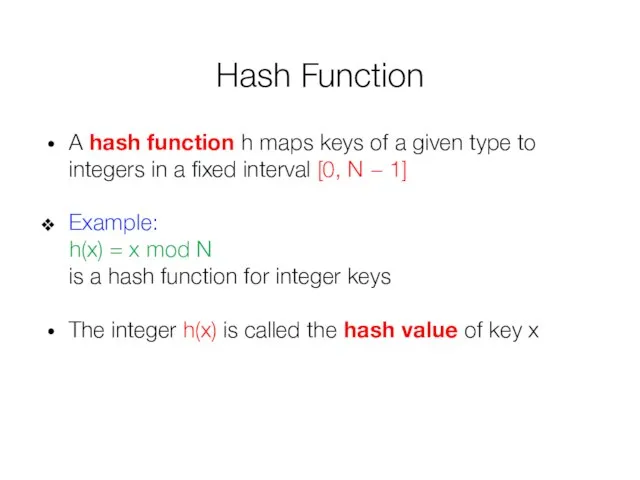
- 23. Hash Function A hash function h maps keys of a given type to integers in a
- 24. Simple Hash Function for Integers
- 25. General Hash Functions A hash function is usually specified as the composition of two functions: Hash
- 26. Parts of a Hash Function © 2014 Goodrich, Tamassia, Goldwasser
- 27. Ideal Hash Function Every resulting hash value has exactly one input that will produce it Same
- 28. Some Principles If n items are placed in m buckets, and n is greater than m,
- 29. Collisions So collisions are inevitable Our goal should therefore be to minimize collisions We will achieve
- 30. Tip! Designing a hash function is a black art It is always better to use a
- 31. Hash Codes Memory address: We reinterpret the memory address of the key object as an integer
- 32. Hash Codes (cont.) Integer cast: We reinterpret the bits of the key as an integer Suitable
- 33. Hash Codes (cont.) Component sum: We partition the bits of the key into components of fixed
- 34. Hash Codes (cont.) We partition the bits of the key into a sequence of components of
- 35. Compression Functions Division: h2 (y) = y mod N The size N of the hash table
- 36. Compression Functions Multiply, Add and Divide (MAD) h2 (y) = [(ay + b) mod p] mod
- 37. Collision Handling
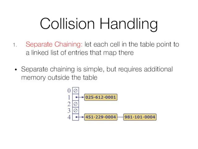
- 38. Collision Handling Separate Chaining: let each cell in the table point to a linked list of
- 39. Analysis of get(k) in Separate Chaining
- 40. Analysis of get(k) in Separate Chaining
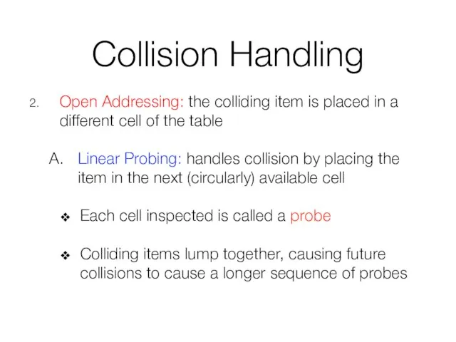
- 41. Collision Handling Open Addressing: the colliding item is placed in a different cell of the table
- 42. Example Example: Linear probing h(x) = x mod 13 Insert keys 18, 41, 22, 44, 59,
- 43. Example Example: Linear probing h(x) = x mod 13 Insert keys 18, 41, 22, 44, 59,
- 44. Search with Linear Probing Consider a hash table A that uses linear probing get(k) We start
- 45. Updates with Linear Probing To handle insertions and deletions, we introduce a special object, called DEFUNCT,
- 46. Updates with Linear Probing put(k, o) We throw an exception if the table is full We
- 47. Collision Handling Open Addressing: the colliding item is placed in a different cell of the table
- 48. Double Hashing The secondary hash function cannot have zero values The table size N must be
- 49. Double Hashing Common choice of compression function for the secondary hash function: d(k) = q −
- 50. Example Consider a hash table storing integer keys that handles collision with double hashing N =
- 51. Example Consider a hash table storing integer keys that handles collision with double hashing N =
- 52. Analysis of get(k) in Open Addressing
- 54. Скачать презентацию
Recap
Elementary data structures
ADT
Array based vs. linked implementation
Worst case time complexity to
Recap
Elementary data structures
ADT
Array based vs. linked implementation
Worst case time complexity to
Today’s Objectives
What is a “MAP or Dictionary ADT”?
What choices do we
Today’s Objectives
What is a “MAP or Dictionary ADT”?
What choices do we

Map or Dictionary
Map or Dictionary
Map or Dictionary
Models a searchable dynamic set of key-value entries
Main operations
Map or Dictionary
Models a searchable dynamic set of key-value entries
Main operations
The Map ADT
get(k): if the map M has an entry with
The Map ADT
get(k): if the map M has an entry with
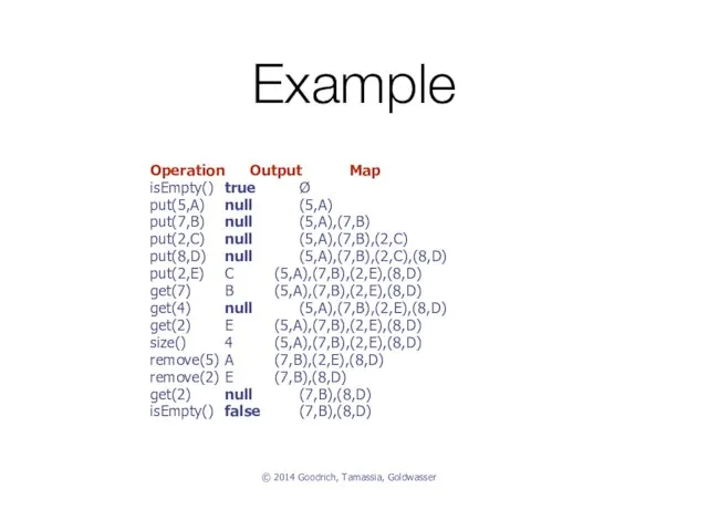
Example
Operation Output Map
isEmpty() true Ø
put(5,A) null (5,A)
put(7,B) null (5,A),(7,B)
put(2,C) null (5,A),(7,B),(2,C)
put(8,D) null (5,A),(7,B),(2,C),(8,D)
put(2,E) C (5,A),(7,B),(2,E),(8,D)
get(7) B (5,A),(7,B),(2,E),(8,D)
get(4) null (5,A),(7,B),(2,E),(8,D)
get(2) E (5,A),(7,B),(2,E),(8,D)
size() 4 (5,A),(7,B),(2,E),(8,D)
remove(5) A (7,B),(2,E),(8,D)
remove(2) E (7,B),(8,D)
get(2) null (7,B),(8,D)
isEmpty() false (7,B),(8,D)
© 2014 Goodrich, Tamassia, Goldwasser
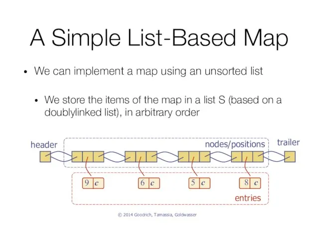
A Simple List-Based Map
We can implement a map using an unsorted
A Simple List-Based Map
We can implement a map using an unsorted
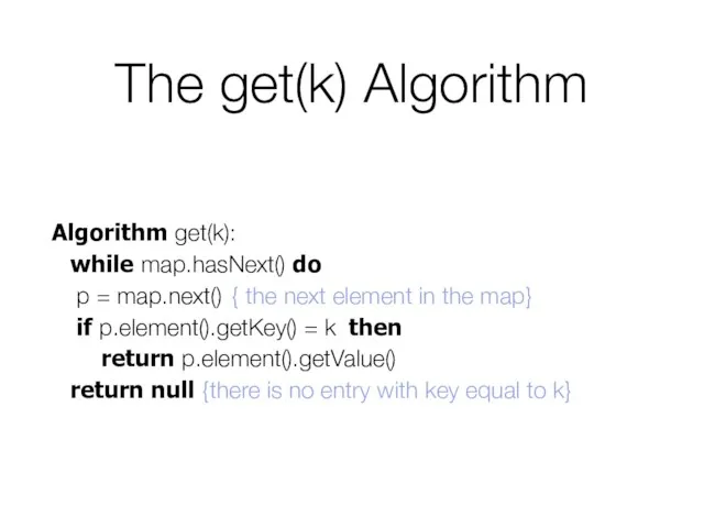
The get(k) Algorithm
Algorithm get(k):
while map.hasNext() do
p = map.next() { the next
The get(k) Algorithm
Algorithm get(k):
while map.hasNext() do
p = map.next() { the next
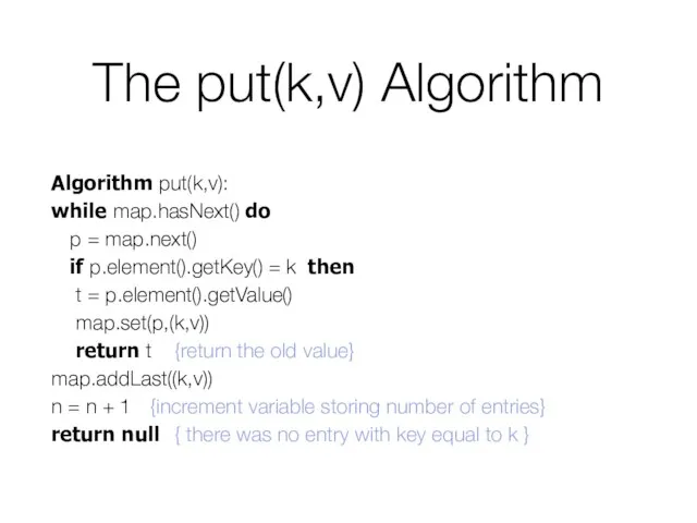
The put(k,v) Algorithm
Algorithm put(k,v):
while map.hasNext() do
p = map.next()
if p.element().getKey() = k
The put(k,v) Algorithm
Algorithm put(k,v):
while map.hasNext() do
p = map.next()
if p.element().getKey() = k
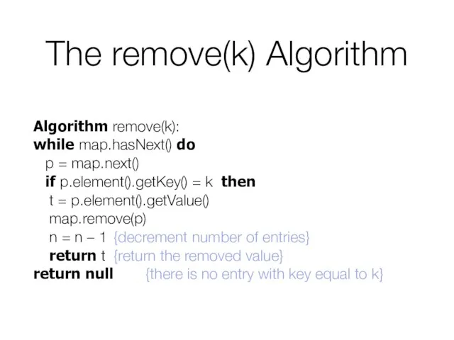
The remove(k) Algorithm
Algorithm remove(k):
while map.hasNext() do
p = map.next()
if p.element().getKey() = k
The remove(k) Algorithm
Algorithm remove(k):
while map.hasNext() do
p = map.next()
if p.element().getKey() = k
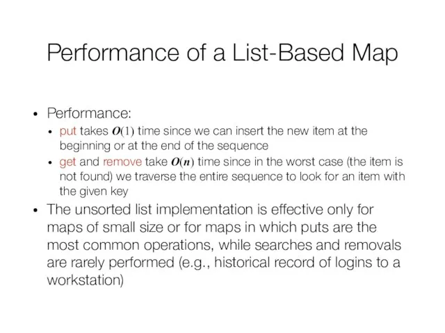
Performance of a List-Based Map
Performance:
put takes O(1) time since we can
Performance of a List-Based Map
Performance:
put takes O(1) time since we can

Hash Map
Hash Map

Let’s Start With this Question
How much time does it take to
Let’s Start With this Question
How much time does it take to
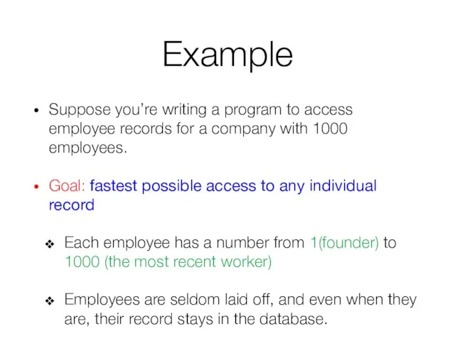
Example
Suppose you’re writing a program to access employee records for a
Example
Suppose you’re writing a program to access employee records for a
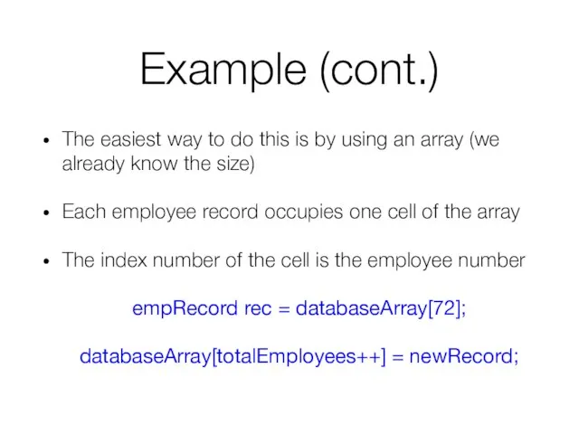
Example (cont.)
The easiest way to do this is by using an
Example (cont.)
The easiest way to do this is by using an
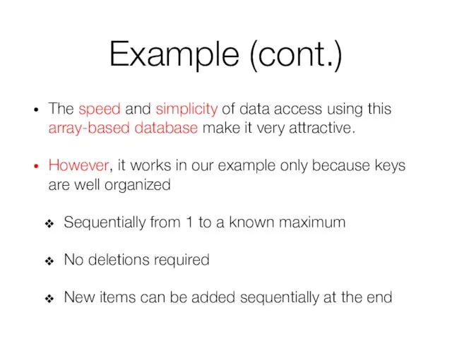
Example (cont.)
The speed and simplicity of data access using this array-based
Example (cont.)
The speed and simplicity of data access using this array-based
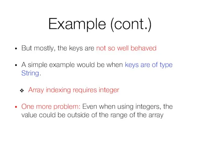
Example (cont.)
But mostly, the keys are not so well behaved
A simple
Example (cont.)
But mostly, the keys are not so well behaved
A simple
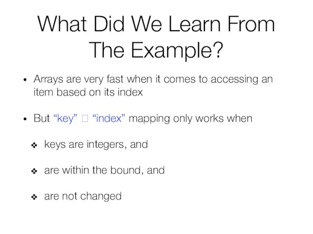
What Did We Learn From The Example?
Arrays are very fast when
What Did We Learn From The Example?
Arrays are very fast when
Hash Map
Hash Table is a very practical way to maintain a
Hash Map
Hash Table is a very practical way to maintain a
Hash Table
Hash Table
Hash Table
Hash Table
Hash Function
A hash function h maps keys of a given type
Hash Function
A hash function h maps keys of a given type
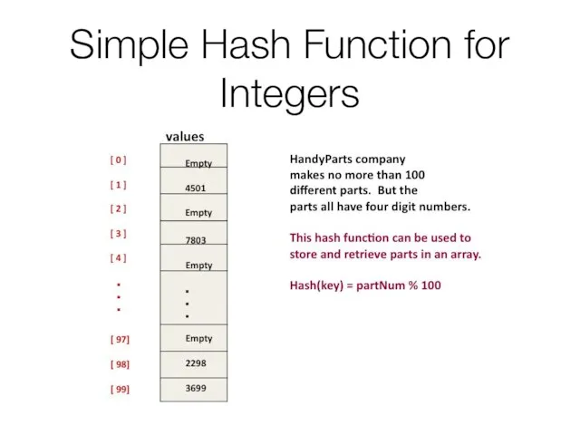
Simple Hash Function for Integers
Simple Hash Function for Integers
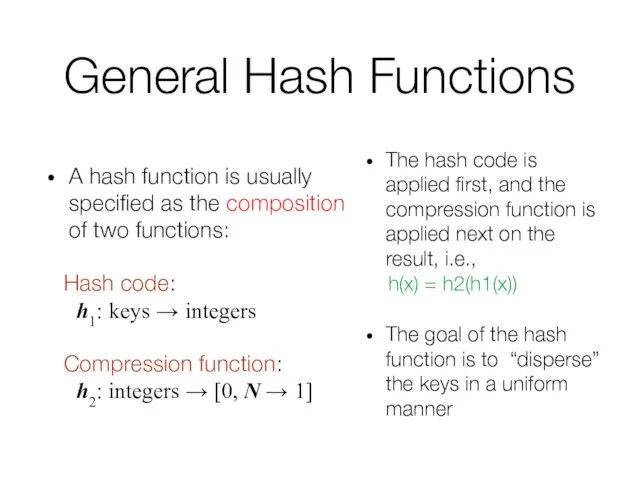
General Hash Functions
A hash function is usually specified as the composition
General Hash Functions
A hash function is usually specified as the composition
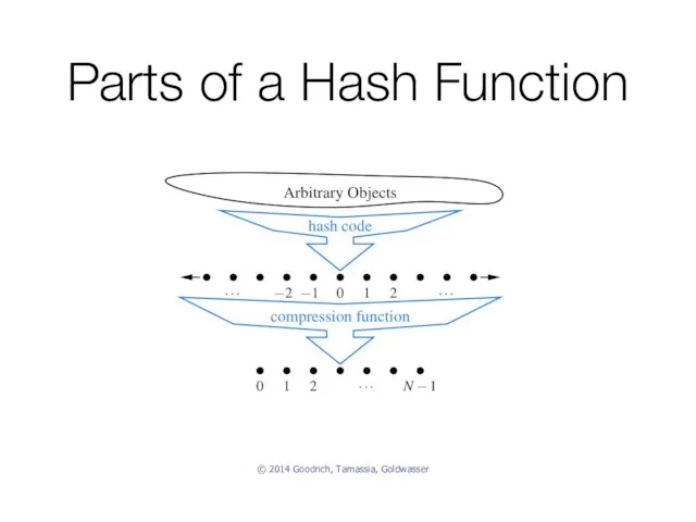
Parts of a Hash Function
© 2014 Goodrich, Tamassia, Goldwasser
Parts of a Hash Function
© 2014 Goodrich, Tamassia, Goldwasser
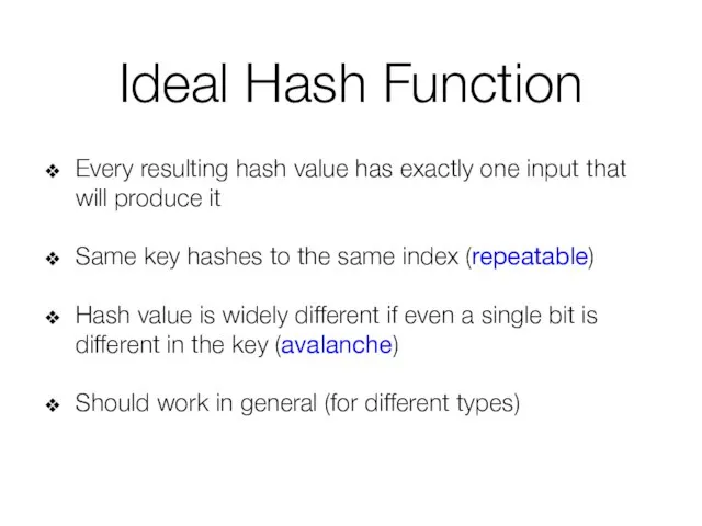
Ideal Hash Function
Every resulting hash value has exactly one input that
Ideal Hash Function
Every resulting hash value has exactly one input that
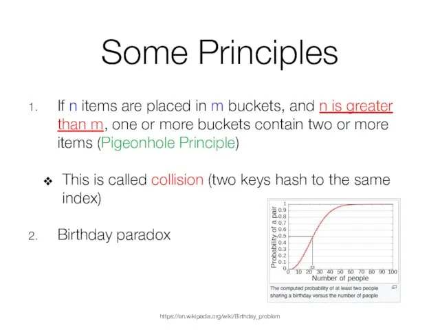
Some Principles
If n items are placed in m buckets, and n
Some Principles
If n items are placed in m buckets, and n
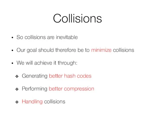
Collisions
So collisions are inevitable
Our goal should therefore be to minimize collisions
We
Collisions
So collisions are inevitable
Our goal should therefore be to minimize collisions
We
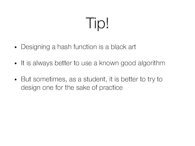
Tip!
Designing a hash function is a black art
It is always better
Tip!
Designing a hash function is a black art
It is always better
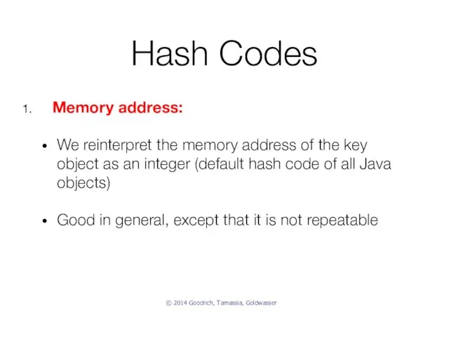
Hash Codes
Memory address:
We reinterpret the memory address of the key object
Hash Codes
Memory address:
We reinterpret the memory address of the key object
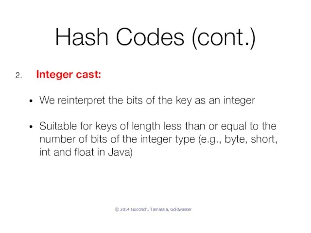
Hash Codes (cont.)
Integer cast:
We reinterpret the bits of the key as
Hash Codes (cont.)
Integer cast:
We reinterpret the bits of the key as
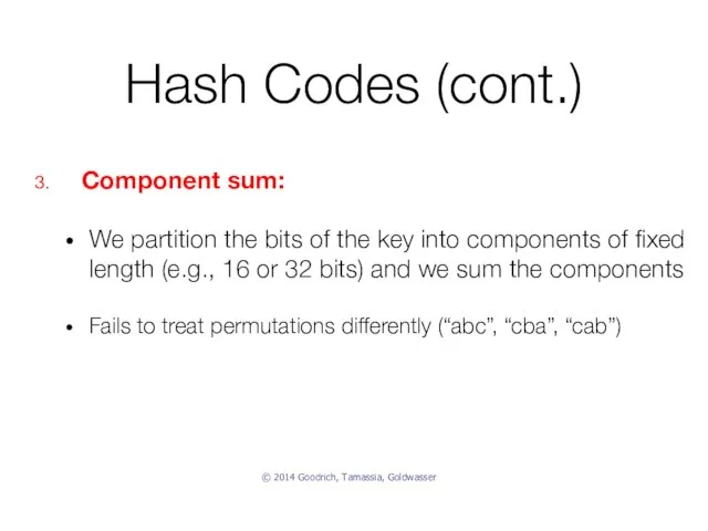
Hash Codes (cont.)
Component sum:
We partition the bits of the key into
Hash Codes (cont.)
Component sum:
We partition the bits of the key into
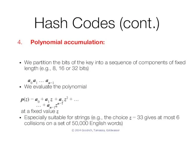
Hash Codes (cont.)
We partition the bits of the key into a
Hash Codes (cont.)
We partition the bits of the key into a
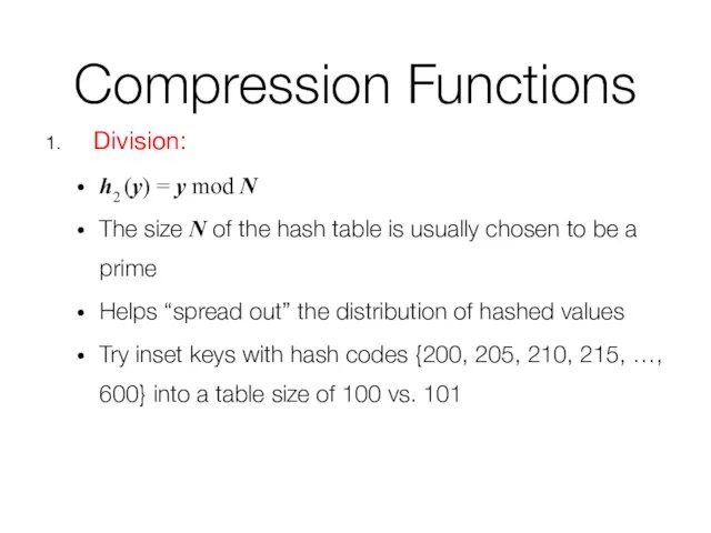
Compression Functions
Division:
h2 (y) = y mod N
The size N of the
Compression Functions
Division:
h2 (y) = y mod N
The size N of the
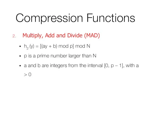
Compression Functions
Multiply, Add and Divide (MAD)
h2 (y) = [(ay + b)
Compression Functions
Multiply, Add and Divide (MAD)
h2 (y) = [(ay + b)
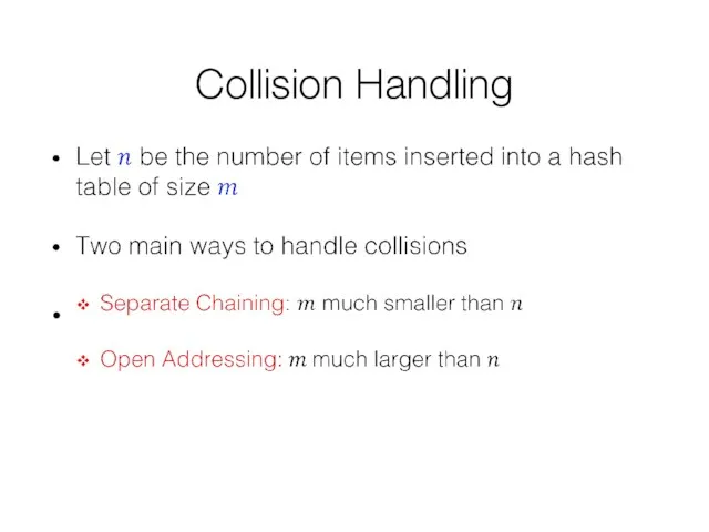
Collision Handling
Collision Handling
Collision Handling
Separate Chaining: let each cell in the table point to
Collision Handling
Separate Chaining: let each cell in the table point to
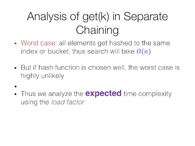
Analysis of get(k) in Separate Chaining
Analysis of get(k) in Separate Chaining
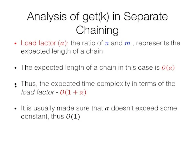
Analysis of get(k) in Separate Chaining
Analysis of get(k) in Separate Chaining
Collision Handling
Open Addressing: the colliding item is placed in a different
Collision Handling
Open Addressing: the colliding item is placed in a different
Example
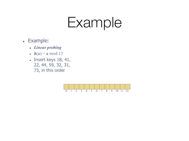
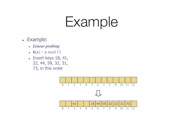
Example:
Linear probing
h(x) = x mod 13
Insert keys 18, 41, 22, 44,
Example
Example:
Linear probing
h(x) = x mod 13
Insert keys 18, 41, 22, 44,
Example
Example:
Linear probing
h(x) = x mod 13
Insert keys 18, 41, 22, 44,
Example
Example:
Linear probing
h(x) = x mod 13
Insert keys 18, 41, 22, 44,
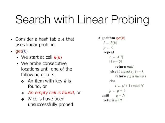
Search with Linear Probing
Consider a hash table A that uses linear
Search with Linear Probing
Consider a hash table A that uses linear
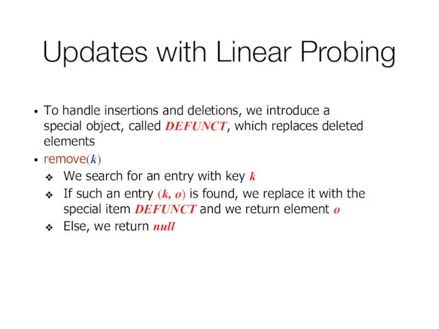
Updates with Linear Probing
To handle insertions and deletions, we introduce a
Updates with Linear Probing
To handle insertions and deletions, we introduce a
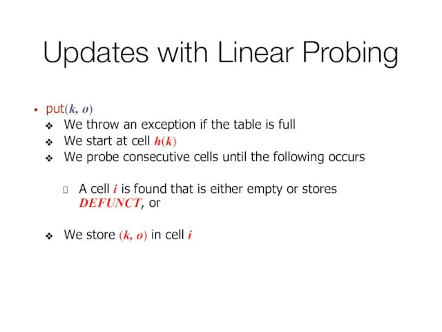
Updates with Linear Probing
put(k, o)
We throw an exception if the table
Updates with Linear Probing
put(k, o)
We throw an exception if the table
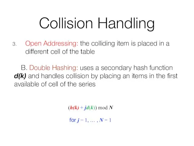
Collision Handling
Open Addressing: the colliding item is placed in a different
Collision Handling
Open Addressing: the colliding item is placed in a different
Double Hashing
The secondary hash function cannot have zero values
The table size
Double Hashing
The secondary hash function cannot have zero values
The table size
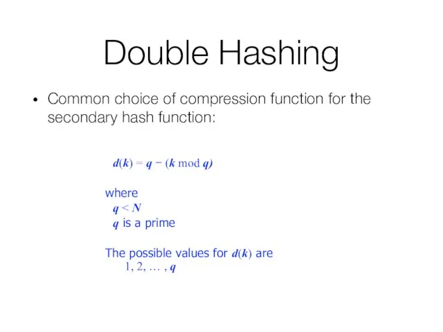
Double Hashing
Common choice of compression function for the secondary hash function:
Double Hashing
Common choice of compression function for the secondary hash function:
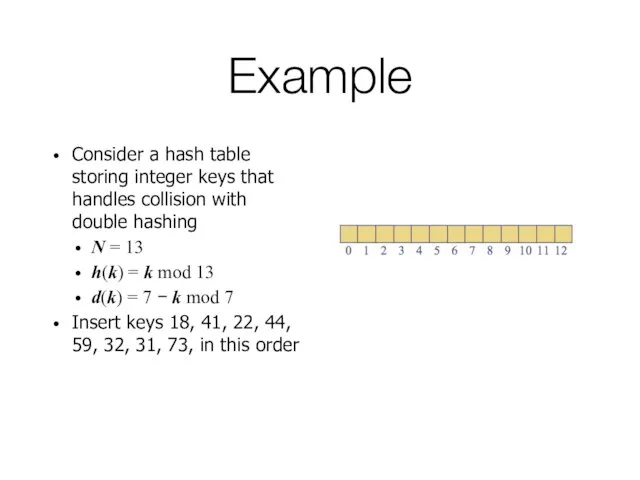
Example
Consider a hash table storing integer keys that handles collision with
Example
Consider a hash table storing integer keys that handles collision with
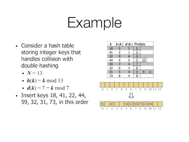
Example
Consider a hash table storing integer keys that handles collision with
Example
Consider a hash table storing integer keys that handles collision with
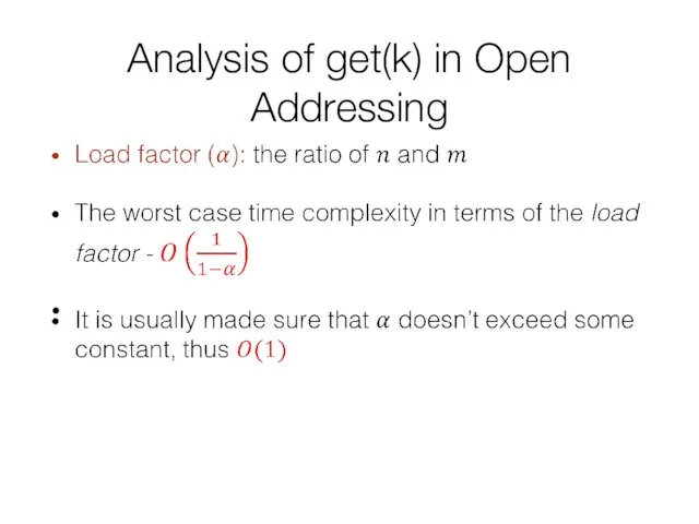
Analysis of get(k) in Open Addressing
Analysis of get(k) in Open Addressing
 Объектно-ориентированное программирование
 Семинар по memory studies
 Деректерді ұсынудың негізгі ұғымдарының дамыуы
 Реестр
 Правовое регулирование взаимоотношений библиотеки и читателей
 Семинар-тренинг 5-8 октября 2014 года. Реестр документов. Документы "Интеркампани"
 Технология Вики-Вики и ее использование в сетевом ресурсе «Летописи» Патрина Елена Алексеевна, зам. директора по УВР школы №3 г. К
 新編維修教材
 Аттестационная работа. Программа внеурочной деятельности для 1-4 классов В мир проектов с Перволого
 Информатика в играх и задачах. Основы логики. 2 класс ( 3 урок)
 Data analysis. Data management
 Основы структурного программирования
 Исполнитель Черепаха. Построение рисунков на плоскости
 Запросы к нескольким таблицам. Работа с SQL
 Школьники и Интернет. Новые информационные возможности и новые угрозы
 Возможности социальных медиа и перспективы их использования
 Презентация "Исследование физических моделей" - скачать презентации по Информатике
 Распределенные базы данных. Лекция 13
 Логичесие функциив в Excel
 Виды и классификация промышленных сетей
 Подготовка электронных материалов. Требования к оформлению текстовых документов
 Аттестационная работа. Применение метода учебных проектов при обучении информатики в начальных классах
 Смартфон в житті. Застосування в життєвих ситуаціях
 Основные этапы программирования как науки
 Классы. Конструкторы и деструкторы
 Массивы
 Служба резервного копирования и восстановления Symantec Backup Exec. Крок
 Сложение чисел в обратном и дополнительном кодах