- Dense Linear Algebra: History and Structure, Parallel Matrix Multiplication

Содержание
- 2. 02/22/2011 CS267 Lecture 11 Outline History and motivation Structure of the Dense Linear Algebra motif Parallel
- 3. 02/22/2011 CS267 Lecture 11 Outline History and motivation Structure of the Dense Linear Algebra motif Parallel
- 4. Motifs The Motifs (formerly “Dwarfs”) from “The Berkeley View” (Asanovic et al.) Motifs form key computational
- 5. What is dense linear algebra? Not just matmul! Linear Systems: Ax=b Least Squares: choose x to
- 6. A brief history of (Dense) Linear Algebra software (1/7) Libraries like EISPACK (for eigenvalue problems) Then
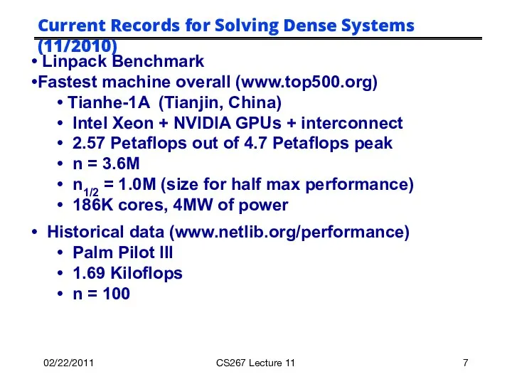
- 7. 02/22/2011 CS267 Lecture 11 Current Records for Solving Dense Systems (11/2010) Linpack Benchmark Fastest machine overall
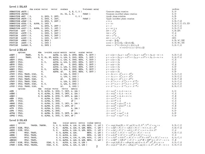
- 8. A brief history of (Dense) Linear Algebra software (2/7) But the BLAS-1 weren’t enough Consider AXPY
- 9. A brief history of (Dense) Linear Algebra software (3/7) The next step: BLAS-3 (1987-1988) Standard library
- 10. 02/25/2009 CS267 Lecture 8
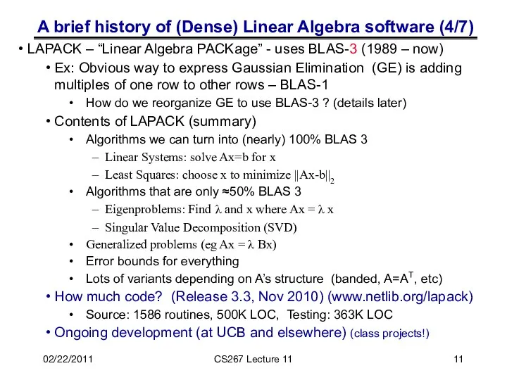
- 11. A brief history of (Dense) Linear Algebra software (4/7) LAPACK – “Linear Algebra PACKage” - uses
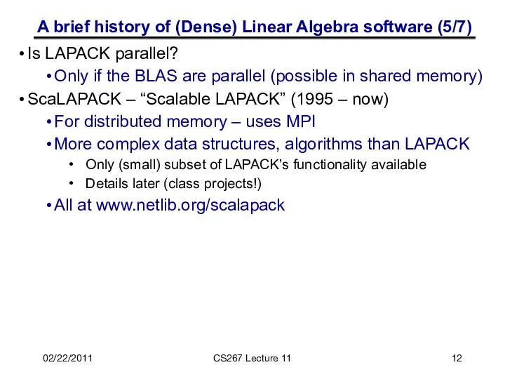
- 12. A brief history of (Dense) Linear Algebra software (5/7) Is LAPACK parallel? Only if the BLAS
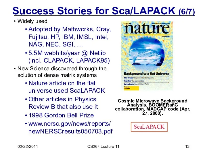
- 13. 02/22/2011 CS267 Lecture 11 Success Stories for Sca/LAPACK (6/7) Cosmic Microwave Background Analysis, BOOMERanG collaboration, MADCAP
- 14. Back to basics: Why avoiding communication is important (1/2) Algorithms have two costs: Arithmetic (FLOPS) Communication:
- 15. Why avoiding communication is important (2/2) Running time of an algorithm is sum of 3 terms:
- 16. for i = 1 to n {read row i of A into fast memory, n2 reads}
- 17. Less Communication with Blocked Matrix Multiply Blocked Matmul C = A·B explicitly refers to subblocks of
- 18. Blocked vs Cache-Oblivious Algorithms Blocked Matmul C = A·B explicitly refers to subblocks of A, B
- 19. Communication Lower Bounds: Prior Work on Matmul Assume n3 algorithm (i.e. not Strassen-like) Sequential case, with
- 20. New lower bound for all “direct” linear algebra Holds for BLAS, LU, QR, eig, SVD, tensor
- 21. Can we attain these lower bounds? Do conventional dense algorithms as implemented in LAPACK and ScaLAPACK
- 22. A brief future look at (Dense) Linear Algebra software (7/7) PLASMA and MAGMA (now) Planned extensions
- 23. 02/22/2011 CS267 Lecture 11 Outline History and motivation Structure of the Dense Linear Algebra motif Parallel
- 24. What could go into the linear algebra motif(s)? For all linear algebra problems For all matrix/problem
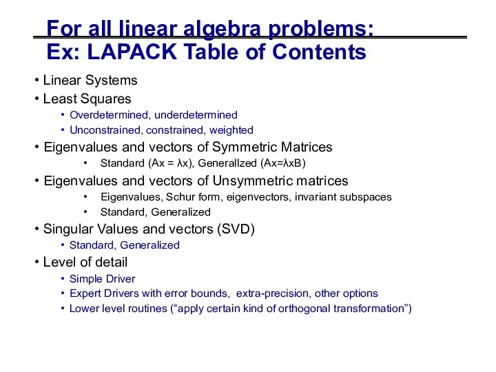
- 25. For all linear algebra problems: Ex: LAPACK Table of Contents Linear Systems Least Squares Overdetermined, underdetermined
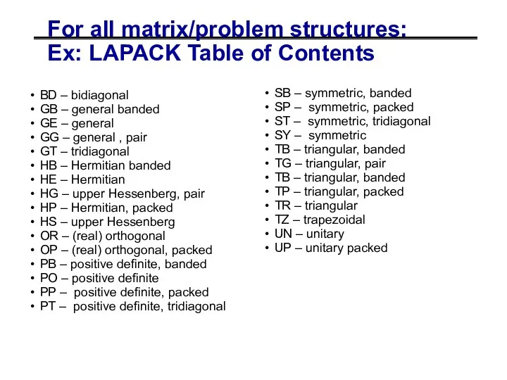
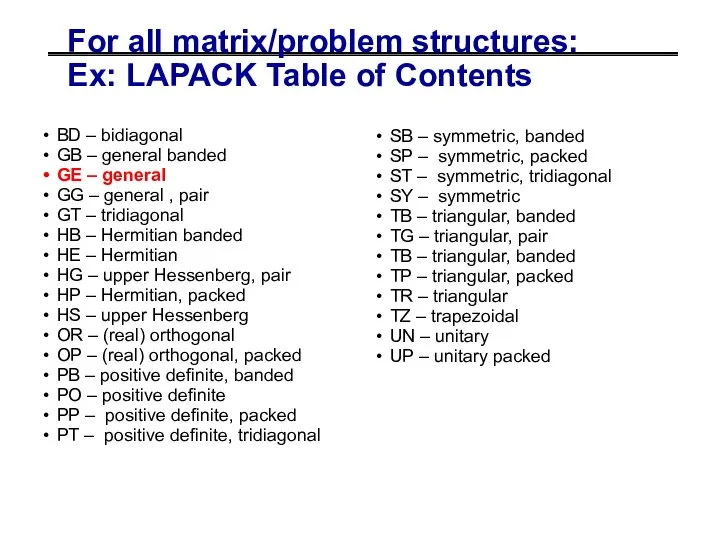
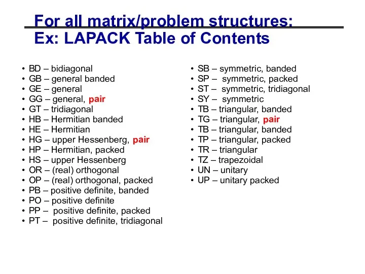
- 26. For all matrix/problem structures: Ex: LAPACK Table of Contents BD – bidiagonal GB – general banded
- 27. For all matrix/problem structures: Ex: LAPACK Table of Contents BD – bidiagonal GB – general banded
- 28. For all matrix/problem structures: Ex: LAPACK Table of Contents BD – bidiagonal GB – general banded
- 29. For all matrix/problem structures: Ex: LAPACK Table of Contents BD – bidiagonal GB – general banded
- 30. For all matrix/problem structures: Ex: LAPACK Table of Contents BD – bidiagonal GB – general banded
- 31. For all matrix/problem structures: Ex: LAPACK Table of Contents BD – bidiagonal GB – general banded
- 32. For all matrix/problem structures: Ex: LAPACK Table of Contents BD – bidiagonal GB – general banded
- 33. For all matrix/problem structures: Ex: LAPACK Table of Contents BD – bidiagonal GB – general banded
- 34. Organizing Linear Algebra – in books www.netlib.org/lapack www.netlib.org/scalapack www.cs.utk.edu/~dongarra/etemplates www.netlib.org/templates gams.nist.gov
- 35. 02/22/2011 CS267 Lecture 11 Outline History and motivation Structure of the Dense Linear Algebra motif Parallel
- 36. 02/22/2011 CS267 Lecture 11 Different Parallel Data Layouts for Matrices (not all!) 1) 1D Column Blocked
- 37. 02/22/2011 CS267 Lecture 11 Parallel Matrix-Vector Product Compute y = y + A*x, where A is
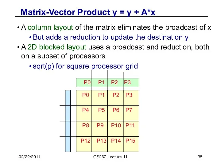
- 38. 02/22/2011 CS267 Lecture 11 Matrix-Vector Product y = y + A*x A column layout of the
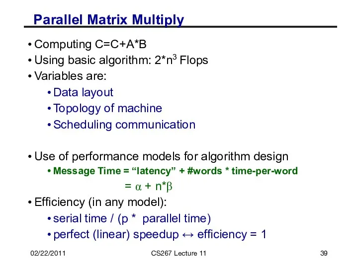
- 39. 02/22/2011 CS267 Lecture 11 Parallel Matrix Multiply Computing C=C+A*B Using basic algorithm: 2*n3 Flops Variables are:
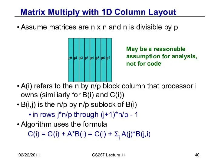
- 40. 02/22/2011 CS267 Lecture 11 Matrix Multiply with 1D Column Layout Assume matrices are n x n
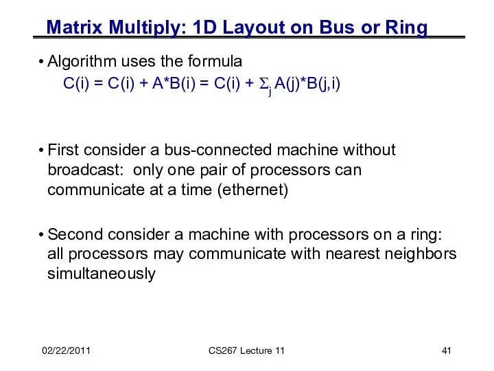
- 41. 02/22/2011 CS267 Lecture 11 Matrix Multiply: 1D Layout on Bus or Ring Algorithm uses the formula
- 42. 02/22/2011 CS267 Lecture 11 MatMul: 1D layout on Bus without Broadcast Naïve algorithm: C(myproc) = C(myproc)
- 43. 02/22/2011 CS267 Lecture 11 Naïve MatMul (continued) Cost of inner loop: computation: 2*n*(n/p)2 = 2*n3/p2 communication:
- 44. 02/22/2011 CS267 Lecture 11 Matmul for 1D layout on a Processor Ring Pairs of adjacent processors
- 45. 02/22/2011 CS267 Lecture 11 Matmul for 1D layout on a Processor Ring Time of inner loop
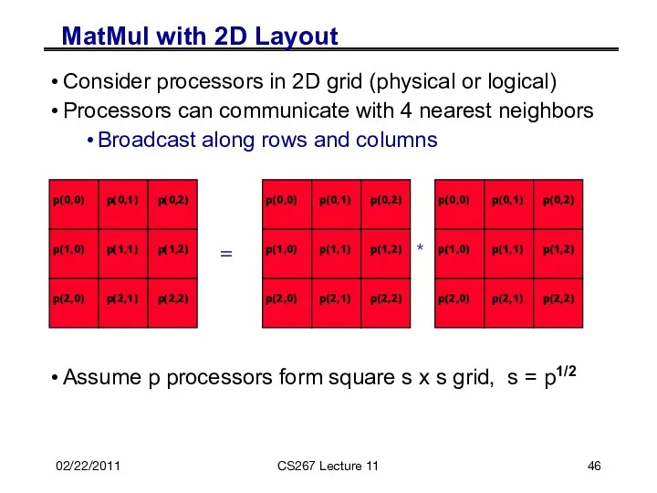
- 46. 02/22/2011 CS267 Lecture 11 MatMul with 2D Layout Consider processors in 2D grid (physical or logical)
- 47. 02/22/2011 CS267 Lecture 11 Cannon’s Algorithm … C(i,j) = C(i,j) + Σ A(i,k)*B(k,j) … assume s
- 48. 02/22/2011 CS267 Lecture 11 C(1,2) = A(1,0) * B(0,2) + A(1,1) * B(1,2) + A(1,2) *
- 49. 02/22/2011 CS267 Lecture 11 Initial Step to Skew Matrices in Cannon Initial blocked input After skewing
- 50. 02/22/2011 CS267 Lecture 11 Skewing Steps in Cannon All blocks of A must multiply all like-colored
- 51. 02/22/2011 CS267 Lecture 11 Cost of Cannon’s Algorithm forall i=0 to s-1 … recall s =
- 52. Cannon’s Algorithm is “optimal” Optimal means Considering only O(n3) matmul algs (not Strassen) Considering only O(n2/p)
- 53. 02/22/2011 CS267 Lecture 11 Pros and Cons of Cannon So what if it’s “optimal”, is it
- 54. 02/22/2011 CS267 Lecture 11 SUMMA Algorithm SUMMA = Scalable Universal Matrix Multiply Slightly less efficient, but
- 55. 02/22/2011 CS267 Lecture 11 SUMMA * = i j A(i,k) k k B(k,j) i, j represent
- 56. 02/22/2011 CS267 Lecture 11 SUMMA For k=0 to n/b-1 … where b is the block size
- 57. 02/22/2011 CS267 Lecture 11 SUMMA performance For k=0 to n/b-1 for all i = 1 to
- 58. 02/22/2011 CS267 Lecture 11 SUMMA performance Total time = 2*n3/p + α * log p *
- 59. 02/22/2011 CS267 Lecture 8 PDGEMM = PBLAS routine for matrix multiply Observations: For fixed N, as
- 60. 02/22/2011 CS267 Lecture 11 Summary of Parallel Matrix Multiplication so far 1D Layout Bus without broadcast
- 61. 02/22/2011 CS267 Lecture 11 Summary of Parallel Matrix Multiplication so far 1D Layout Bus without broadcast
- 62. Beating #words_moved = Ω(n2/P1/2) “3D Matmul” Algorithm on P1/3 x P1/3 x P1/3 processor grid Broadcast
- 63. 2.5D algorithms – for c copies 3D 2.5D If 1 ≤ c ≤ p1/3 and M
- 64. 2.5D matrix multiply Interpolate between Cannon and 3D matmul Replicate A, B c-1 times Do p1/2/c3/2
- 65. 2.5D matrix multiply performance Source: Edgar Solomonik
- 66. 02/22/2011 CS267 Lecture 11 ScaLAPACK Parallel Library
- 67. 02/22/2011 CS267 Lecture 11 Extra Slides
- 68. 2/27/08 CS267 Guest Lecture 1 Recursive Layouts For both cache hierarchies and parallelism, recursive layouts may
- 69. 02/09/2006 CS267 Lecture 8 Gaussian Elimination 0 x x x x . . . Standard Way
- 70. 02/09/2006 CS267 Lecture 8 LU Algorithm: 1: Split matrix into two rectangles (m x n/2) if
- 71. 02/09/2006 CS267 Lecture 8 Recursive Factorizations Just as accurate as conventional method Same number of operations
- 72. 02/09/2006 CS267 Lecture 8 LAPACK Recursive LU Recursive LU LAPACK Dual-processor Uniprocessor Slide source: Dongarra
- 73. 02/09/2006 CS267 Lecture 8 Review: BLAS 3 (Blocked) GEPP for ib = 1 to n-1 step
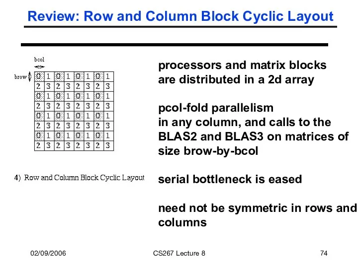
- 74. 02/09/2006 CS267 Lecture 8 Review: Row and Column Block Cyclic Layout processors and matrix blocks are
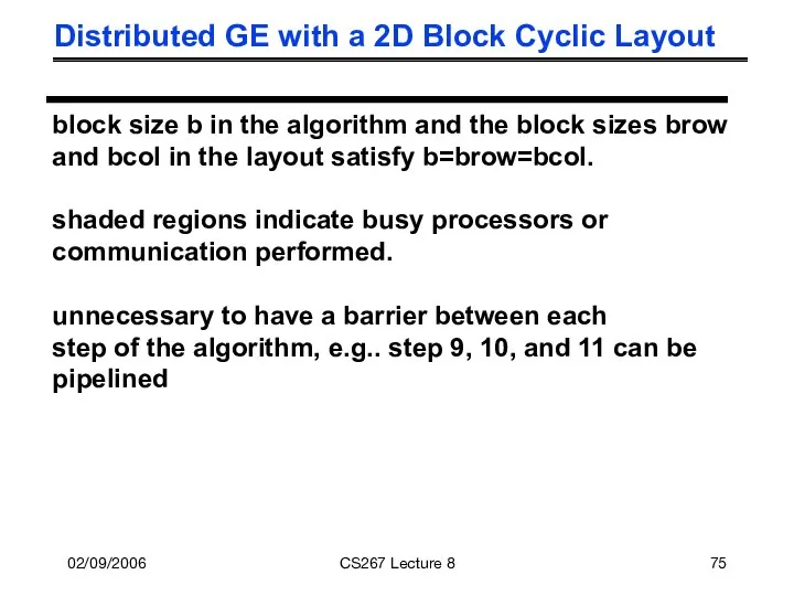
- 75. 02/09/2006 CS267 Lecture 8 Distributed GE with a 2D Block Cyclic Layout block size b in
- 76. 02/09/2006 CS267 Lecture 8 Distributed GE with a 2D Block Cyclic Layout
- 77. 02/09/2006 CS267 Lecture 8 Matrix multiply of green = green - blue * pink
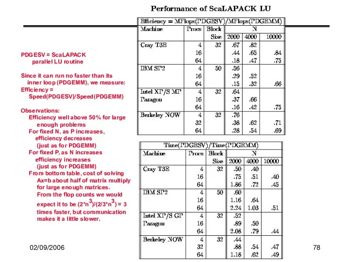
- 78. 02/09/2006 CS267 Lecture 8 PDGESV = ScaLAPACK parallel LU routine Since it can run no faster
- 79. 02/09/2006 CS267 Lecture 8
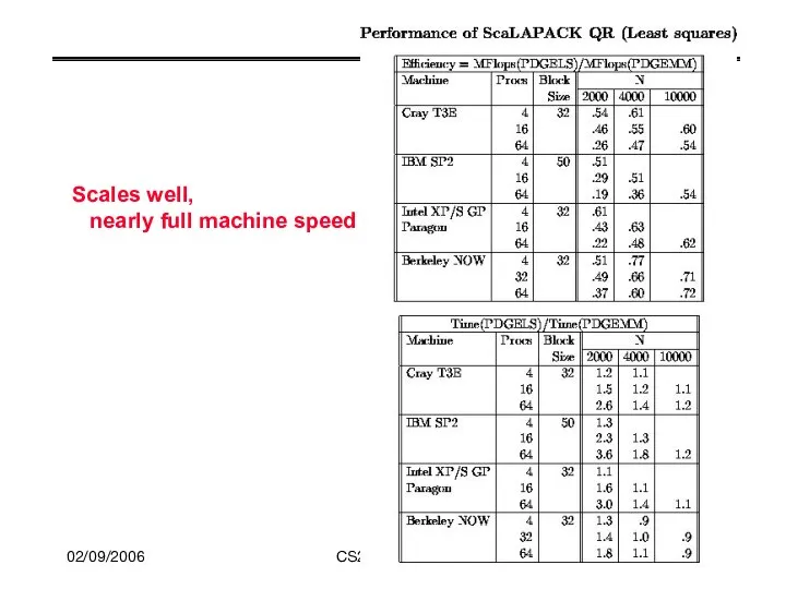
- 80. 02/09/2006 CS267 Lecture 8 Scales well, nearly full machine speed
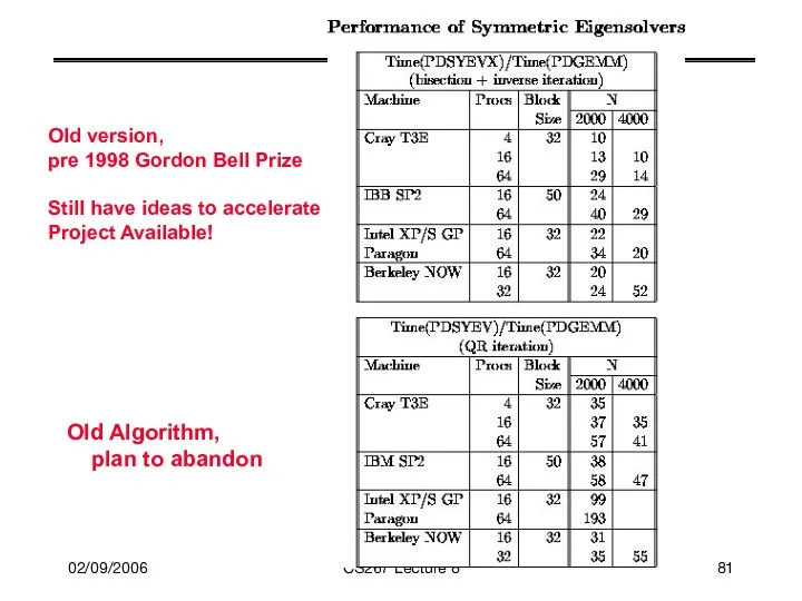
- 81. 02/09/2006 CS267 Lecture 8 Old version, pre 1998 Gordon Bell Prize Still have ideas to accelerate
- 82. 02/09/2006 CS267 Lecture 8 Have good ideas to speedup Project available! Hardest of all to parallelize
- 83. 02/09/2006 CS267 Lecture 8 Out-of-core means matrix lives on disk; too big for main mem Much
- 84. 02/09/2006 CS267 Lecture 8 A small software project ...
- 85. 02/09/2006 CS267 Lecture 8 Work-Depth Model of Parallelism The work depth model: The simplest model is
- 86. 02/09/2006 CS267 Lecture 8 Latency Bandwidth Model Network of fixed number P of processors fully connected
- 87. 02/09/2006 CS267 Lecture 8 Initial Step to Skew Matrices in Cannon Initial blocked input After skewing
- 88. 02/09/2006 CS267 Lecture 8 Skewing Steps in Cannon First step Second Third A(0,1) A(0,2) A(1,0) A(2,0)
- 89. 2/25/2009 CS267 Lecture 8 Motivation (1) 3 Basic Linear Algebra Problems Linear Equations: Solve Ax=b for
- 90. 2/25/2009 CS267 Lecture 8 Motivation (2) Why dense A, as opposed to sparse A? Many large
- 91. 02/25/2009 CS267 Lecture 8 Algorithms for 2D (3D) Poisson Equation (N = n2 (n3) vars) Algorithm
- 92. Lessons and Questions (1) Structure of the problem matters Cost of solution can vary dramatically (n3
- 93. Organizing Linear Algebra (1) By Operations Low level (eg mat-mul: BLAS) Standard level (eg solve Ax=b,
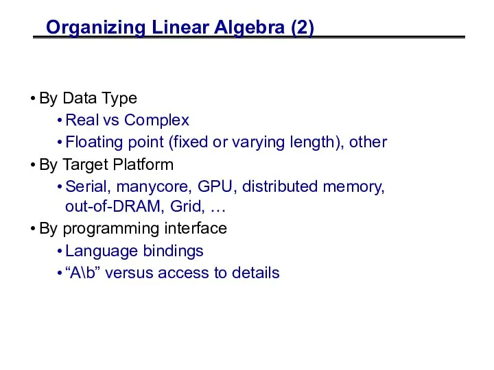
- 94. Organizing Linear Algebra (2) By Data Type Real vs Complex Floating point (fixed or varying length),
- 95. For all linear algebra problems: Ex: LAPACK Table of Contents Linear Systems Least Squares Overdetermined, underdetermined
- 96. For all matrix/problem structures: Ex: LAPACK Table of Contents BD – bidiagonal GB – general banded
- 97. For all matrix/problem structures: Ex: LAPACK Table of Contents BD – bidiagonal GB – general banded
- 98. For all matrix/problem structures: Ex: LAPACK Table of Contents BD – bidiagonal GB – general banded
- 99. For all matrix/problem structures: Ex: LAPACK Table of Contents BD – bidiagonal GB – general banded
- 100. For all matrix/problem structures: Ex: LAPACK Table of Contents BD – bidiagonal GB – general banded
- 101. For all matrix/problem structures: Ex: LAPACK Table of Contents BD – bidiagonal GB – general banded
- 102. For all matrix/problem structures: Ex: LAPACK Table of Contents BD – bidiagonal GB – general banded
- 103. For all data types: Ex: LAPACK Table of Contents Real and complex Single and double precision
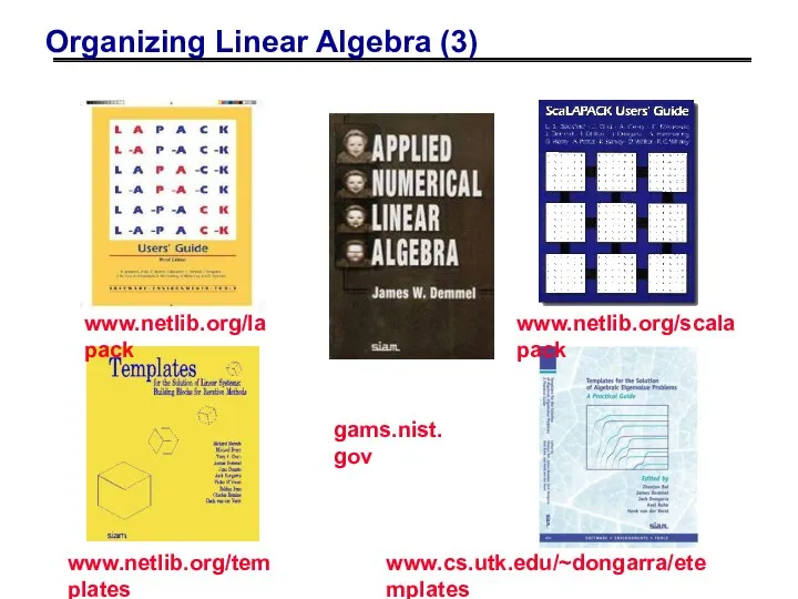
- 104. Organizing Linear Algebra (3) www.netlib.org/lapack www.netlib.org/scalapack www.cs.utk.edu/~dongarra/etemplates www.netlib.org/templates gams.nist.gov
- 106. Скачать презентацию
02/22/2011
CS267 Lecture 11
Outline
History and motivation
Structure of the Dense Linear Algebra motif
Parallel
02/22/2011
CS267 Lecture 11
Outline
History and motivation
Structure of the Dense Linear Algebra motif
Parallel
02/22/2011
CS267 Lecture 11
Outline
History and motivation
Structure of the Dense Linear Algebra motif
Parallel
02/22/2011
CS267 Lecture 11
Outline
History and motivation
Structure of the Dense Linear Algebra motif
Parallel
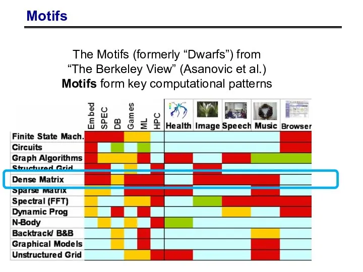
Motifs
The Motifs (formerly “Dwarfs”) from
“The Berkeley View” (Asanovic et al.)
Motifs
Motifs
The Motifs (formerly “Dwarfs”) from
“The Berkeley View” (Asanovic et al.)
Motifs
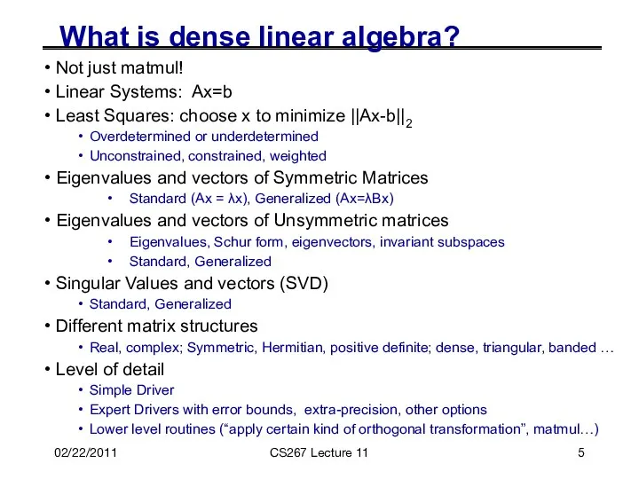
What is dense linear algebra?
Not just matmul!
Linear Systems: Ax=b
Least Squares: choose
What is dense linear algebra?
Not just matmul!
Linear Systems: Ax=b
Least Squares: choose
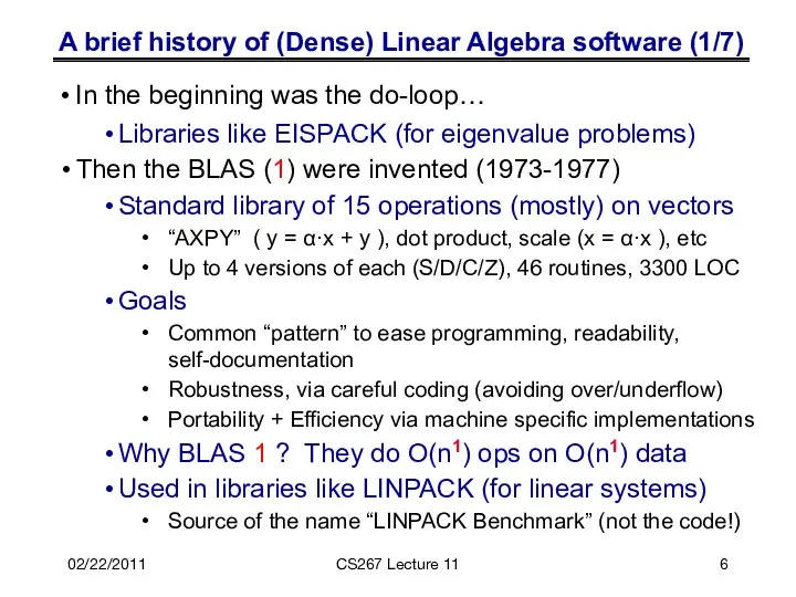
A brief history of (Dense) Linear Algebra software (1/7)
Libraries like EISPACK
A brief history of (Dense) Linear Algebra software (1/7)
Libraries like EISPACK
02/22/2011
CS267 Lecture 11
Current Records for Solving Dense Systems (11/2010)
Linpack Benchmark
02/22/2011
CS267 Lecture 11
Current Records for Solving Dense Systems (11/2010)
Linpack Benchmark
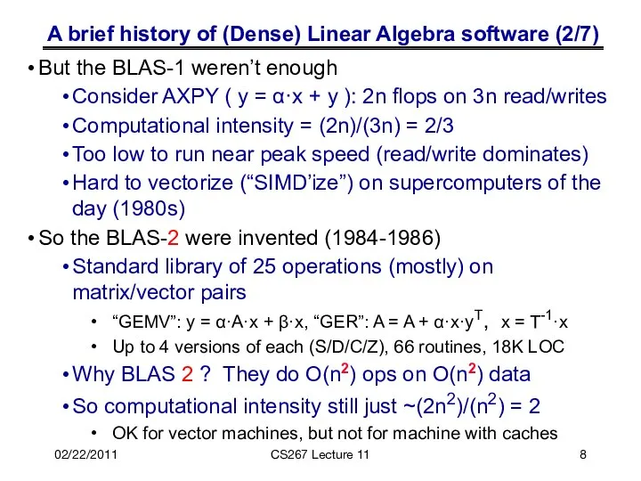
A brief history of (Dense) Linear Algebra software (2/7)
But the BLAS-1
A brief history of (Dense) Linear Algebra software (2/7)
But the BLAS-1
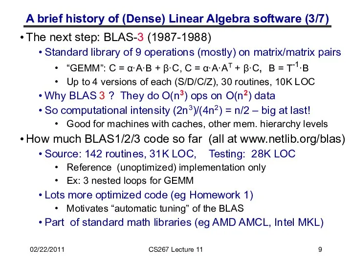
A brief history of (Dense) Linear Algebra software (3/7)
The next step:
A brief history of (Dense) Linear Algebra software (3/7)
The next step:
02/25/2009
CS267 Lecture 8
02/25/2009
CS267 Lecture 8
A brief history of (Dense) Linear Algebra software (4/7)
LAPACK – “Linear
A brief history of (Dense) Linear Algebra software (4/7)
LAPACK – “Linear
A brief history of (Dense) Linear Algebra software (5/7)
Is LAPACK parallel?
Only
A brief history of (Dense) Linear Algebra software (5/7)
Is LAPACK parallel?
Only
02/22/2011
CS267 Lecture 11
Success Stories for Sca/LAPACK (6/7)
Cosmic Microwave Background Analysis, BOOMERanG
02/22/2011
CS267 Lecture 11
Success Stories for Sca/LAPACK (6/7)
Cosmic Microwave Background Analysis, BOOMERanG
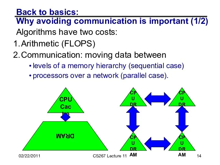
Back to basics:
Why avoiding communication is important (1/2)
Algorithms have two
Back to basics:
Why avoiding communication is important (1/2)
Algorithms have two
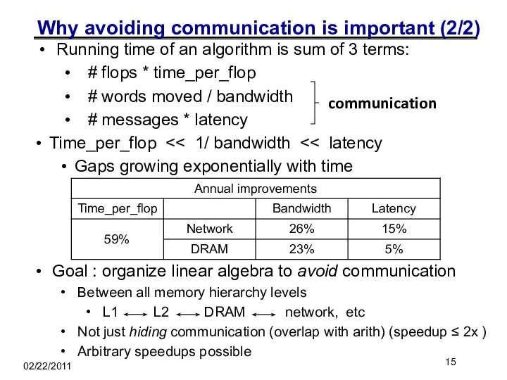
Why avoiding communication is important (2/2)
Running time of an algorithm is
Why avoiding communication is important (2/2)
Running time of an algorithm is
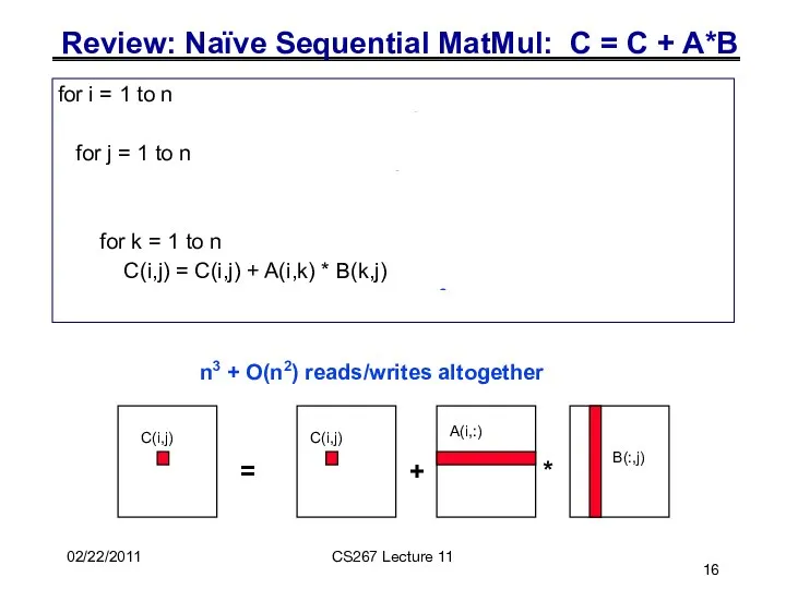
for i = 1 to n
{read row i of A
for i = 1 to n
{read row i of A
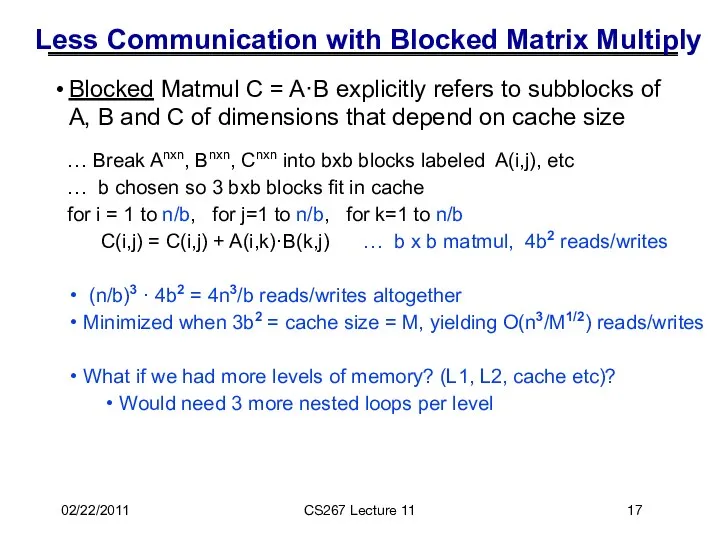
Less Communication with Blocked Matrix Multiply
Blocked Matmul C = A·B explicitly
Less Communication with Blocked Matrix Multiply
Blocked Matmul C = A·B explicitly
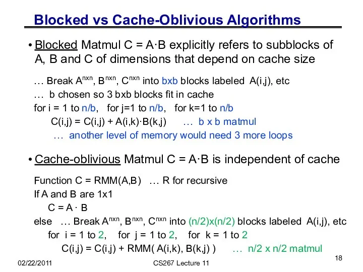
Blocked vs Cache-Oblivious Algorithms
Blocked Matmul C = A·B explicitly refers to
Blocked vs Cache-Oblivious Algorithms
Blocked Matmul C = A·B explicitly refers to
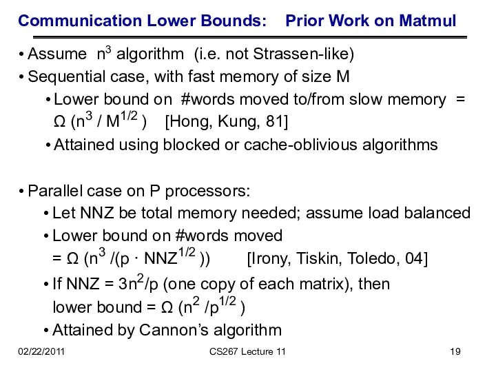
Communication Lower Bounds: Prior Work on Matmul
Assume n3 algorithm (i.e. not
Communication Lower Bounds: Prior Work on Matmul
Assume n3 algorithm (i.e. not
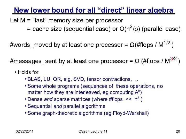
New lower bound for all “direct” linear algebra
Holds for
BLAS, LU, QR,
New lower bound for all “direct” linear algebra
Holds for
BLAS, LU, QR,
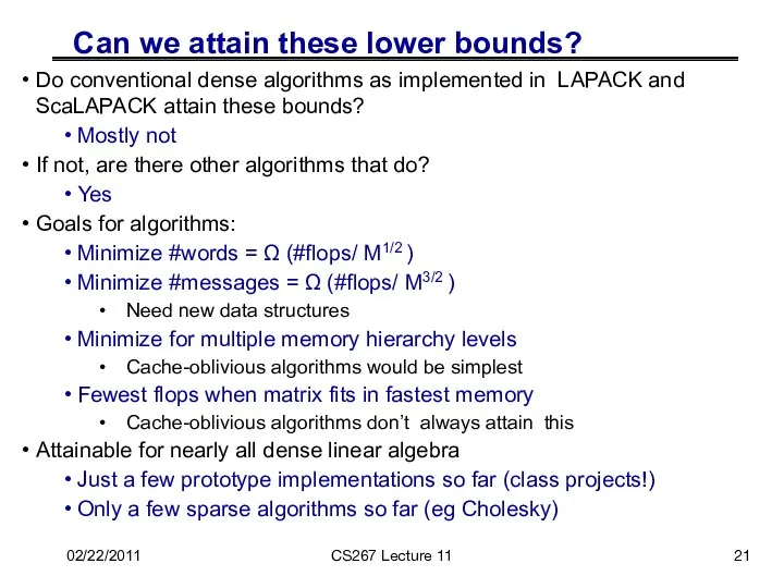
Can we attain these lower bounds?
Do conventional dense algorithms as implemented
Can we attain these lower bounds?
Do conventional dense algorithms as implemented
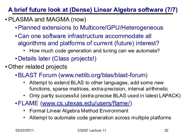
A brief future look at (Dense) Linear Algebra software (7/7)
PLASMA and
A brief future look at (Dense) Linear Algebra software (7/7)
PLASMA and
02/22/2011
CS267 Lecture 11
Outline
History and motivation
Structure of the Dense Linear Algebra motif
Parallel
02/22/2011
CS267 Lecture 11
Outline
History and motivation
Structure of the Dense Linear Algebra motif
Parallel
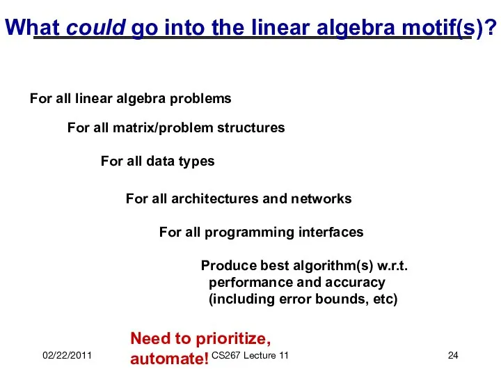
What could go into the linear algebra motif(s)?
For all linear algebra
What could go into the linear algebra motif(s)?
For all linear algebra
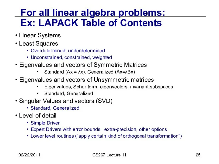
For all linear algebra problems:
Ex: LAPACK Table of Contents
Linear Systems
Least Squares
Overdetermined,
For all linear algebra problems:
Ex: LAPACK Table of Contents
Linear Systems
Least Squares
Overdetermined,
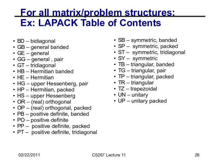
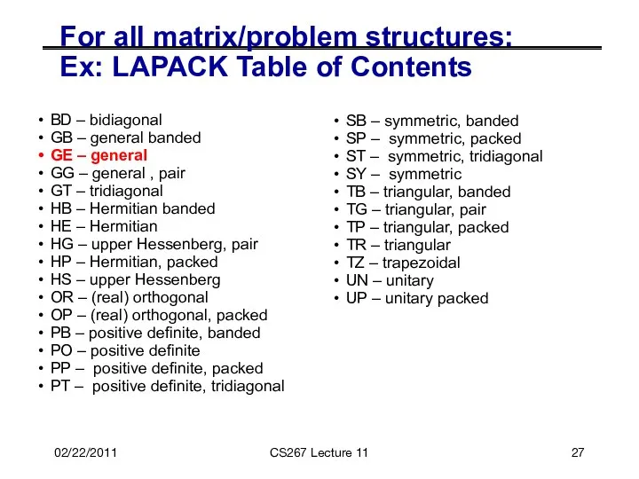
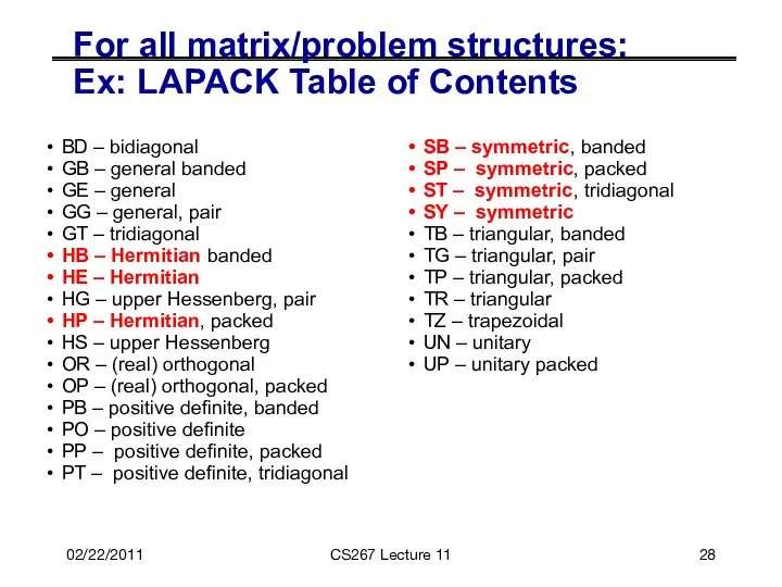
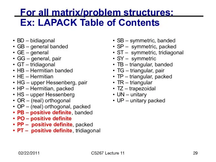
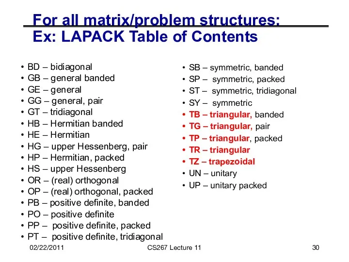
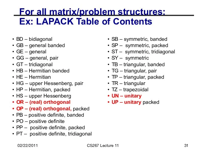
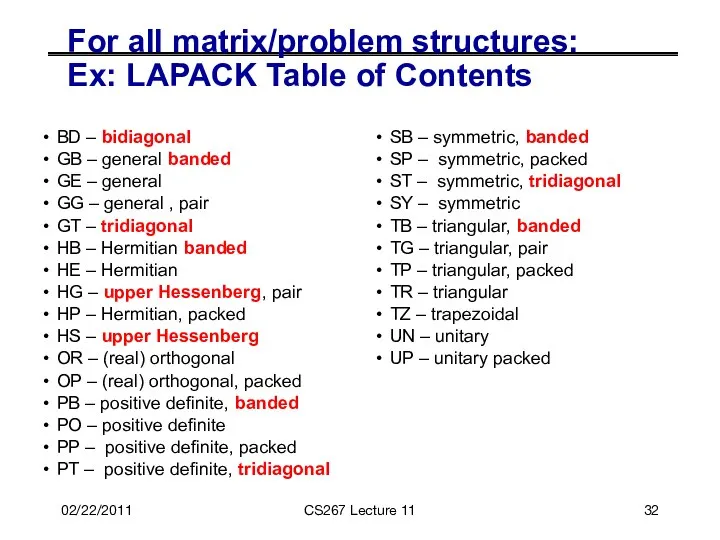
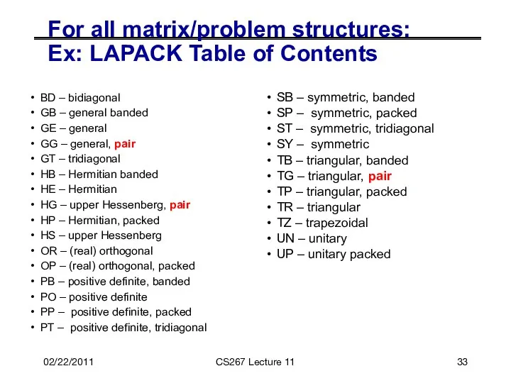
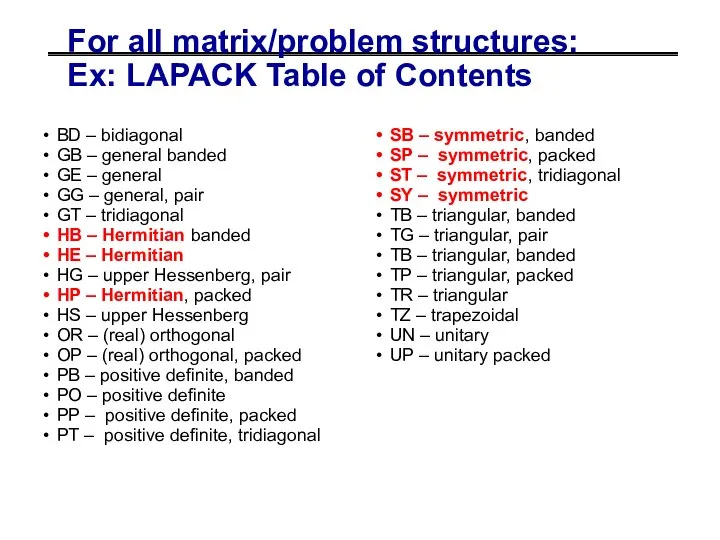
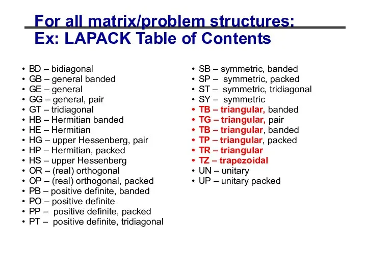
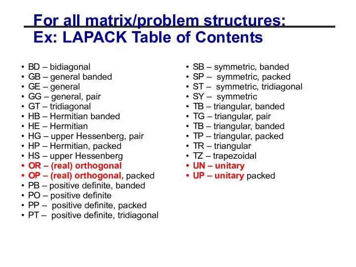
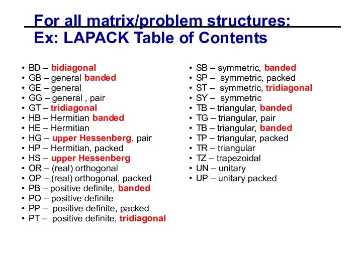
For all matrix/problem structures:
Ex: LAPACK Table of Contents
BD – bidiagonal
GB –
For all matrix/problem structures:
Ex: LAPACK Table of Contents
BD – bidiagonal
GB –
For all matrix/problem structures:
Ex: LAPACK Table of Contents
BD – bidiagonal
GB –
For all matrix/problem structures:
Ex: LAPACK Table of Contents
BD – bidiagonal
GB –
For all matrix/problem structures:
Ex: LAPACK Table of Contents
BD – bidiagonal
GB –
For all matrix/problem structures:
Ex: LAPACK Table of Contents
BD – bidiagonal
GB –
For all matrix/problem structures:
Ex: LAPACK Table of Contents
BD – bidiagonal
GB –
For all matrix/problem structures:
Ex: LAPACK Table of Contents
BD – bidiagonal
GB –
For all matrix/problem structures:
Ex: LAPACK Table of Contents
BD – bidiagonal
GB –
For all matrix/problem structures:
Ex: LAPACK Table of Contents
BD – bidiagonal
GB –
For all matrix/problem structures:
Ex: LAPACK Table of Contents
BD – bidiagonal
GB –
For all matrix/problem structures:
Ex: LAPACK Table of Contents
BD – bidiagonal
GB –
For all matrix/problem structures:
Ex: LAPACK Table of Contents
BD – bidiagonal
GB –
For all matrix/problem structures:
Ex: LAPACK Table of Contents
BD – bidiagonal
GB –
For all matrix/problem structures:
Ex: LAPACK Table of Contents
BD – bidiagonal
GB –
For all matrix/problem structures:
Ex: LAPACK Table of Contents
BD – bidiagonal
GB –
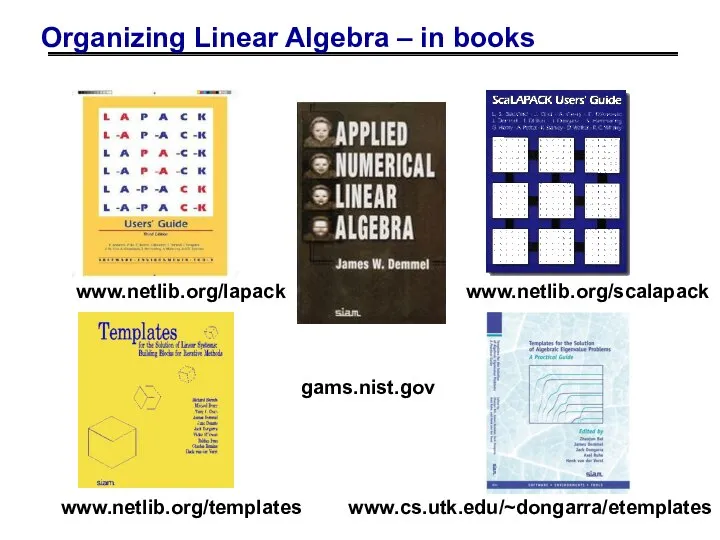
Organizing Linear Algebra – in books
www.netlib.org/lapack
www.netlib.org/scalapack
www.cs.utk.edu/~dongarra/etemplates
www.netlib.org/templates
gams.nist.gov
Organizing Linear Algebra – in books
www.netlib.org/lapack
www.netlib.org/scalapack
www.cs.utk.edu/~dongarra/etemplates
www.netlib.org/templates
gams.nist.gov
02/22/2011
CS267 Lecture 11
Outline
History and motivation
Structure of the Dense Linear Algebra motif
Parallel
02/22/2011
CS267 Lecture 11
Outline
History and motivation
Structure of the Dense Linear Algebra motif
Parallel
02/22/2011
CS267 Lecture 11
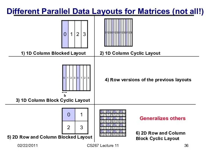
Different Parallel Data Layouts for Matrices (not all!)
1) 1D
02/22/2011
CS267 Lecture 11
Different Parallel Data Layouts for Matrices (not all!)
1) 1D
02/22/2011
CS267 Lecture 11
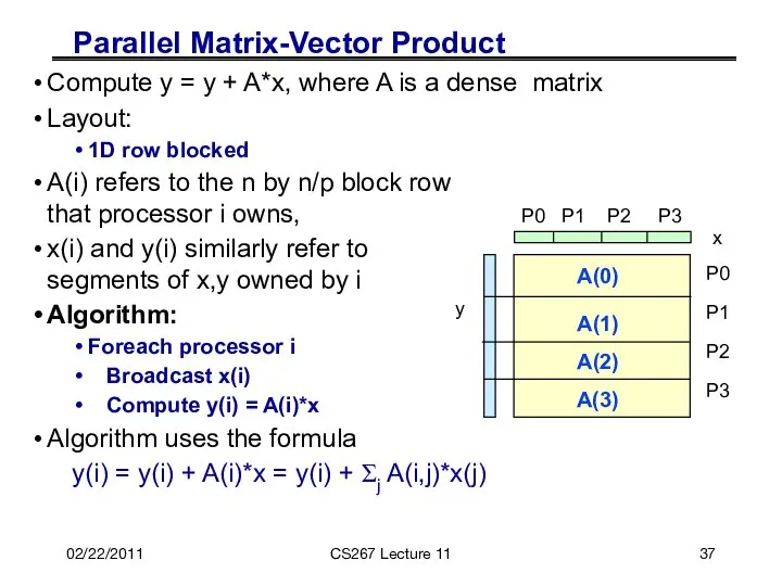
Parallel Matrix-Vector Product
Compute y = y + A*x, where
02/22/2011
CS267 Lecture 11
Parallel Matrix-Vector Product
Compute y = y + A*x, where
02/22/2011
CS267 Lecture 11
Matrix-Vector Product y = y + A*x
A column layout
02/22/2011
CS267 Lecture 11
Matrix-Vector Product y = y + A*x
A column layout
02/22/2011
CS267 Lecture 11
Parallel Matrix Multiply
Computing C=C+A*B
Using basic algorithm: 2*n3 Flops
Variables are:
Data
02/22/2011
CS267 Lecture 11
Parallel Matrix Multiply
Computing C=C+A*B
Using basic algorithm: 2*n3 Flops
Variables are:
Data
02/22/2011
CS267 Lecture 11
Matrix Multiply with 1D Column Layout
Assume matrices are n
02/22/2011
CS267 Lecture 11
Matrix Multiply with 1D Column Layout
Assume matrices are n
02/22/2011
CS267 Lecture 11
Matrix Multiply: 1D Layout on Bus or Ring
Algorithm uses
02/22/2011
CS267 Lecture 11
Matrix Multiply: 1D Layout on Bus or Ring
Algorithm uses
02/22/2011
CS267 Lecture 11
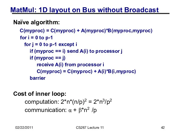
MatMul: 1D layout on Bus without Broadcast
Naïve algorithm:
C(myproc)
02/22/2011
CS267 Lecture 11
MatMul: 1D layout on Bus without Broadcast
Naïve algorithm:
C(myproc)
02/22/2011
CS267 Lecture 11
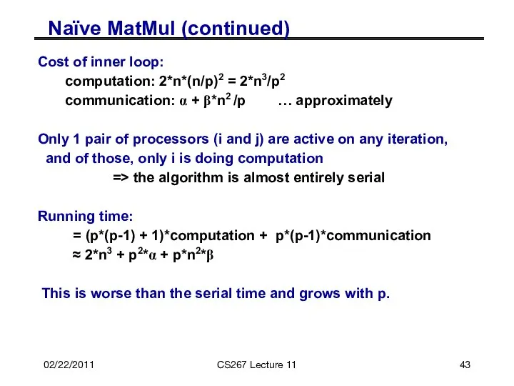
Naïve MatMul (continued)
Cost of inner loop:
computation: 2*n*(n/p)2 =
02/22/2011
CS267 Lecture 11
Naïve MatMul (continued)
Cost of inner loop:
computation: 2*n*(n/p)2 =
02/22/2011
CS267 Lecture 11
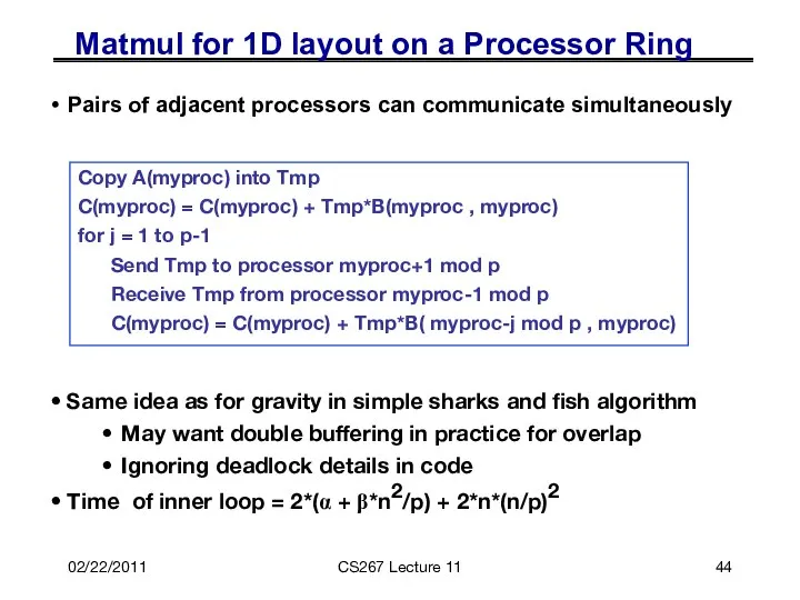
Matmul for 1D layout on a Processor Ring
Pairs of
02/22/2011
CS267 Lecture 11
Matmul for 1D layout on a Processor Ring
Pairs of
02/22/2011
CS267 Lecture 11
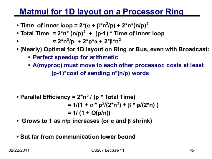
Matmul for 1D layout on a Processor Ring
Time of
02/22/2011
CS267 Lecture 11
Matmul for 1D layout on a Processor Ring
Time of
02/22/2011
CS267 Lecture 11
MatMul with 2D Layout
Consider processors in 2D grid (physical
02/22/2011
CS267 Lecture 11
MatMul with 2D Layout
Consider processors in 2D grid (physical
02/22/2011
CS267 Lecture 11
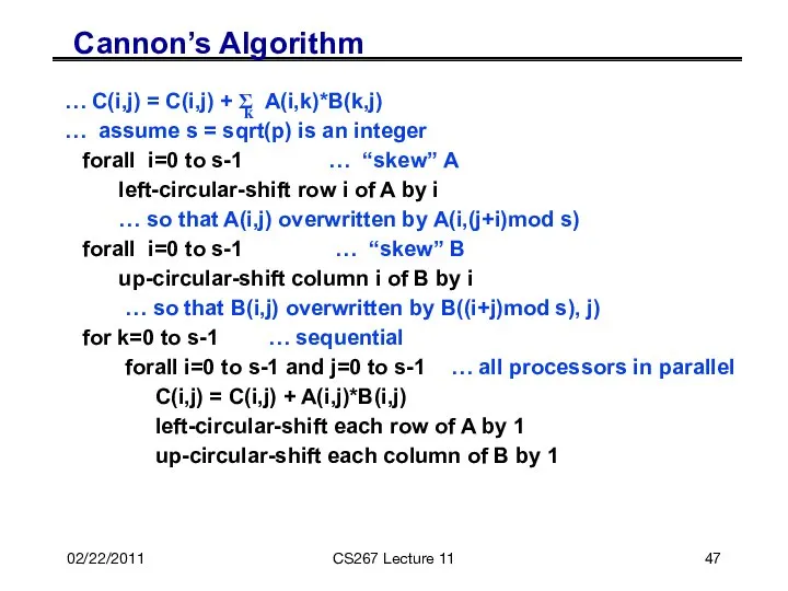
Cannon’s Algorithm
… C(i,j) = C(i,j) + Σ A(i,k)*B(k,j)
… assume
02/22/2011
CS267 Lecture 11
Cannon’s Algorithm
… C(i,j) = C(i,j) + Σ A(i,k)*B(k,j)
… assume
02/22/2011
CS267 Lecture 11
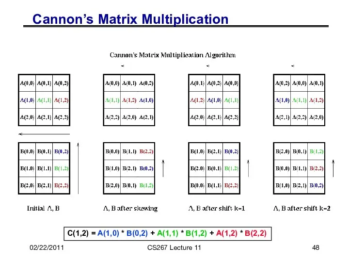
C(1,2) = A(1,0) * B(0,2) + A(1,1) * B(1,2)
02/22/2011
CS267 Lecture 11
C(1,2) = A(1,0) * B(0,2) + A(1,1) * B(1,2)
02/22/2011
CS267 Lecture 11
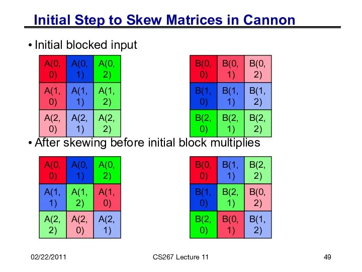
Initial Step to Skew Matrices in Cannon
Initial blocked input
After
02/22/2011
CS267 Lecture 11
Initial Step to Skew Matrices in Cannon
Initial blocked input
After
02/22/2011
CS267 Lecture 11
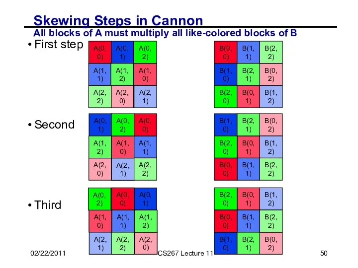
Skewing Steps in Cannon
All blocks of A must multiply
02/22/2011
CS267 Lecture 11
Skewing Steps in Cannon All blocks of A must multiply
02/22/2011
CS267 Lecture 11
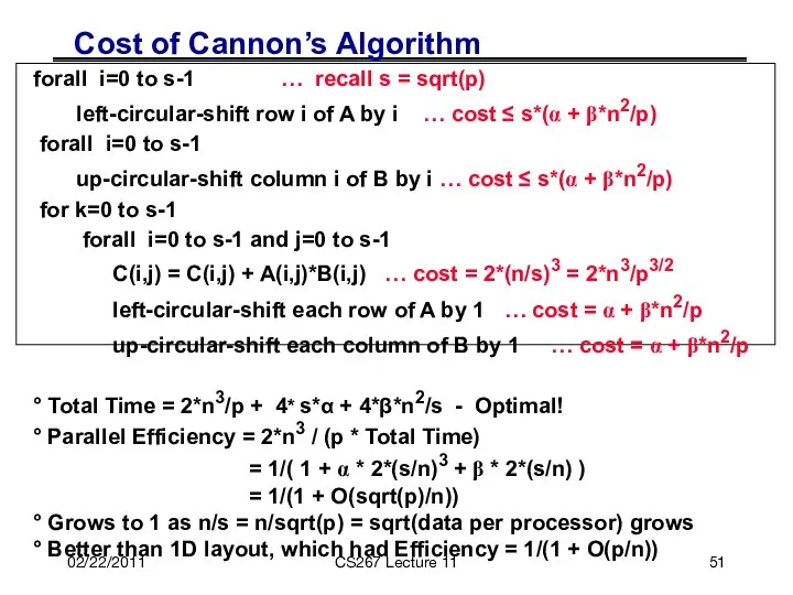
Cost of Cannon’s Algorithm
forall i=0 to s-1 …
02/22/2011
CS267 Lecture 11
Cost of Cannon’s Algorithm
forall i=0 to s-1 …
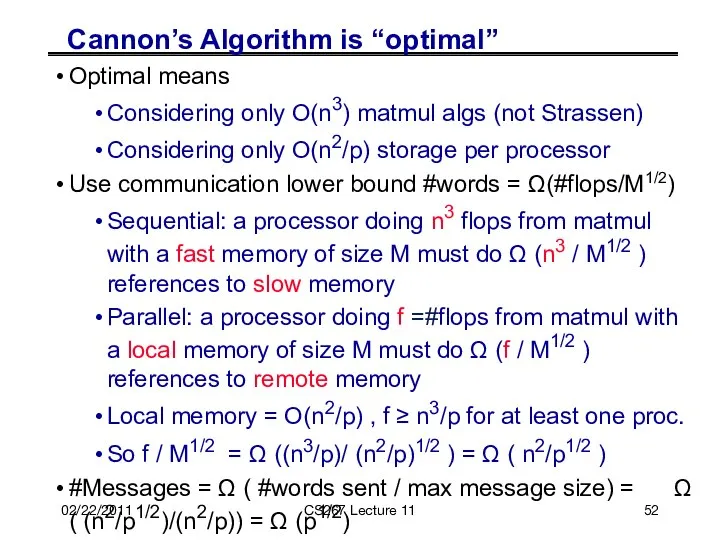
Cannon’s Algorithm is “optimal”
Optimal means
Considering only O(n3) matmul algs (not Strassen)
Considering
Cannon’s Algorithm is “optimal”
Optimal means
Considering only O(n3) matmul algs (not Strassen)
Considering
02/22/2011
CS267 Lecture 11
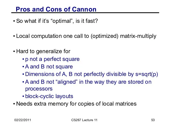
Pros and Cons of Cannon
So what if it’s “optimal”,
02/22/2011
CS267 Lecture 11
Pros and Cons of Cannon
So what if it’s “optimal”,
02/22/2011
CS267 Lecture 11
SUMMA Algorithm
SUMMA = Scalable Universal Matrix Multiply
Slightly less
02/22/2011
CS267 Lecture 11
SUMMA Algorithm
SUMMA = Scalable Universal Matrix Multiply
Slightly less
02/22/2011
CS267 Lecture 11
SUMMA
*
=
i
j
A(i,k)
k
k
B(k,j)
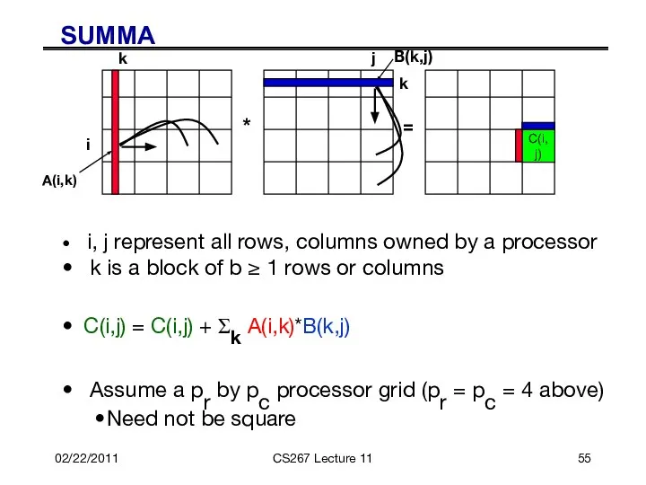
i, j represent all rows, columns
02/22/2011
CS267 Lecture 11
SUMMA
*
=
i
j
A(i,k)
k
k
B(k,j)
i, j represent all rows, columns
02/22/2011
CS267 Lecture 11
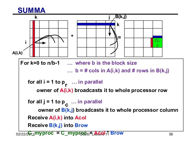
SUMMA
For k=0 to n/b-1 … where b is
02/22/2011
CS267 Lecture 11
SUMMA
For k=0 to n/b-1 … where b is
02/22/2011
CS267 Lecture 11
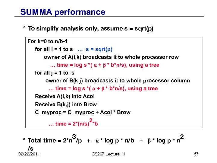
SUMMA performance
For k=0 to n/b-1
for all i
02/22/2011
CS267 Lecture 11
SUMMA performance
For k=0 to n/b-1
for all i
02/22/2011
CS267 Lecture 11
SUMMA performance
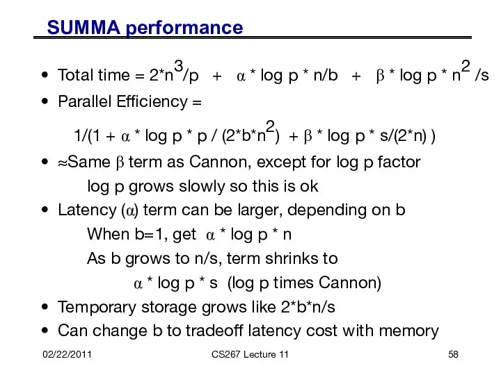
Total time = 2*n3/p + α
02/22/2011
CS267 Lecture 11
SUMMA performance
Total time = 2*n3/p + α
02/22/2011
CS267 Lecture 8
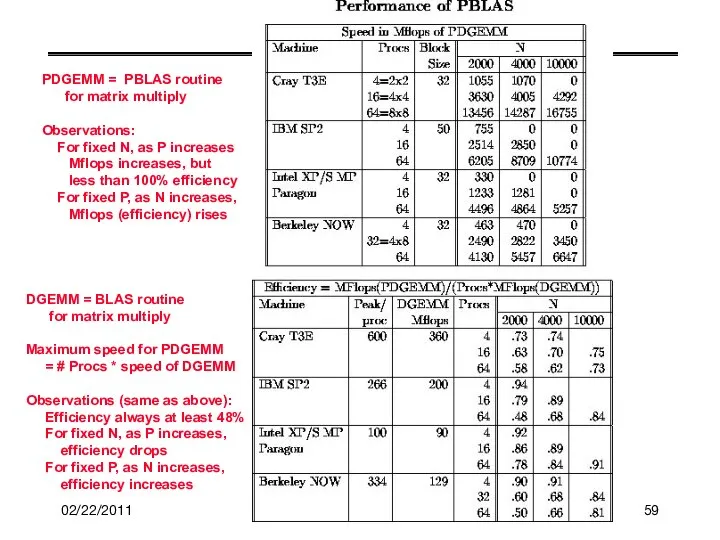
PDGEMM = PBLAS routine
for matrix multiply
Observations:
For fixed
02/22/2011
CS267 Lecture 8
PDGEMM = PBLAS routine
for matrix multiply
Observations:
For fixed
02/22/2011
CS267 Lecture 11
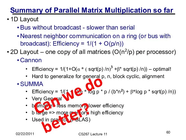
Summary of Parallel Matrix Multiplication so far
1D Layout
Bus without
02/22/2011
CS267 Lecture 11
Summary of Parallel Matrix Multiplication so far
1D Layout
Bus without
02/22/2011
CS267 Lecture 11
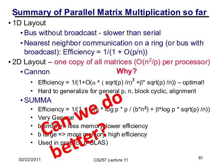
Summary of Parallel Matrix Multiplication so far
1D Layout
Bus without
02/22/2011
CS267 Lecture 11
Summary of Parallel Matrix Multiplication so far
1D Layout
Bus without
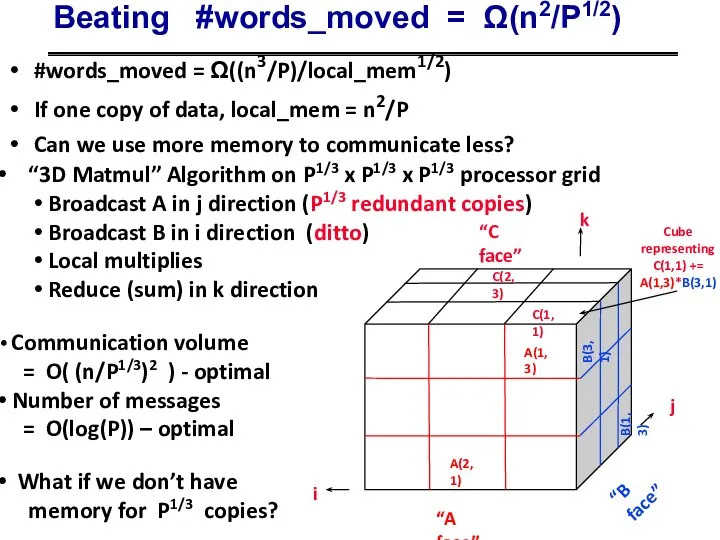
Beating #words_moved = Ω(n2/P1/2)
“3D Matmul” Algorithm on P1/3 x
Beating #words_moved = Ω(n2/P1/2)
“3D Matmul” Algorithm on P1/3 x
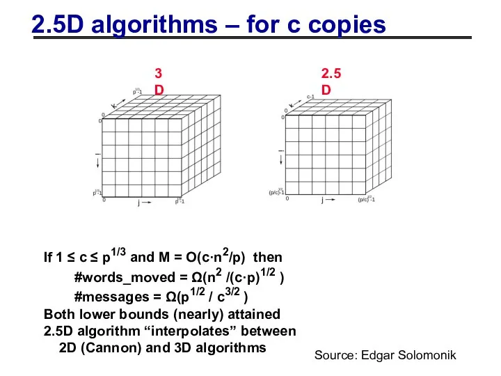
2.5D algorithms – for c copies
3D
2.5D
If 1 ≤ c ≤ p1/3
2.5D algorithms – for c copies
3D
2.5D
If 1 ≤ c ≤ p1/3
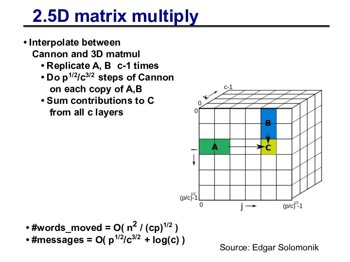
2.5D matrix multiply
Interpolate between
Cannon and 3D matmul
Replicate
2.5D matrix multiply
Interpolate between
Cannon and 3D matmul
Replicate
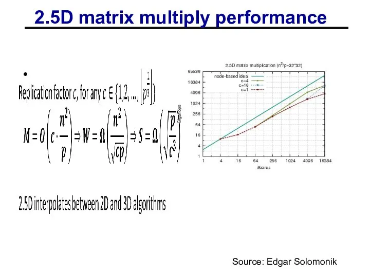
2.5D matrix multiply performance
Source: Edgar Solomonik
2.5D matrix multiply performance
Source: Edgar Solomonik
02/22/2011
CS267 Lecture 11
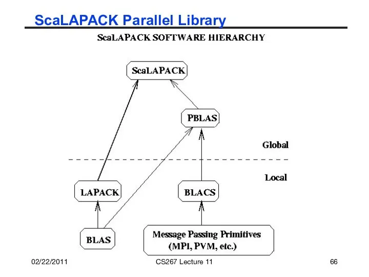
ScaLAPACK Parallel Library
02/22/2011
CS267 Lecture 11
ScaLAPACK Parallel Library
02/22/2011
CS267 Lecture 11
Extra Slides
02/22/2011
CS267 Lecture 11
Extra Slides
2/27/08
CS267 Guest Lecture 1
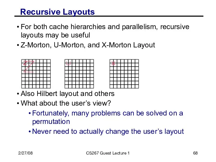
Recursive Layouts
For both cache hierarchies and parallelism, recursive
2/27/08
CS267 Guest Lecture 1
Recursive Layouts
For both cache hierarchies and parallelism, recursive
02/09/2006
CS267 Lecture 8
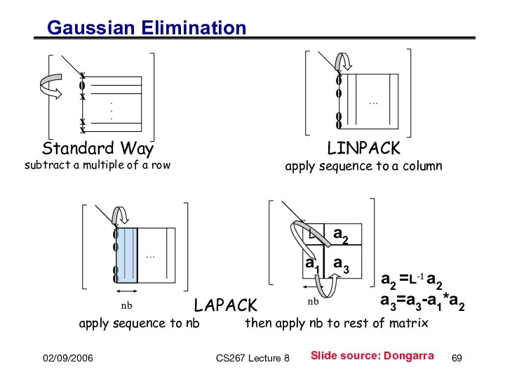
Gaussian Elimination
0
x
x
x
x
.
.
.
Standard Way
subtract a multiple of a row
Slide source:
02/09/2006
CS267 Lecture 8
Gaussian Elimination
0
x
x
x
x
.
.
.
Standard Way
subtract a multiple of a row
Slide source:
02/09/2006
CS267 Lecture 8
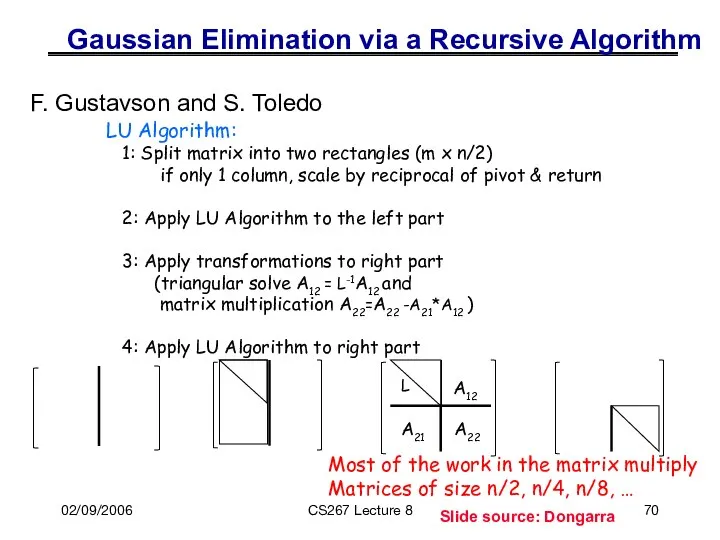
LU Algorithm:
1: Split matrix into two rectangles (m
02/09/2006
CS267 Lecture 8
LU Algorithm:
1: Split matrix into two rectangles (m
02/09/2006
CS267 Lecture 8
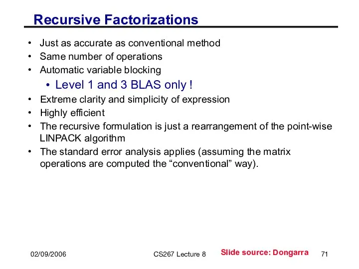
Recursive Factorizations
Just as accurate as conventional method
Same number of
02/09/2006
CS267 Lecture 8
Recursive Factorizations
Just as accurate as conventional method
Same number of
02/09/2006
CS267 Lecture 8
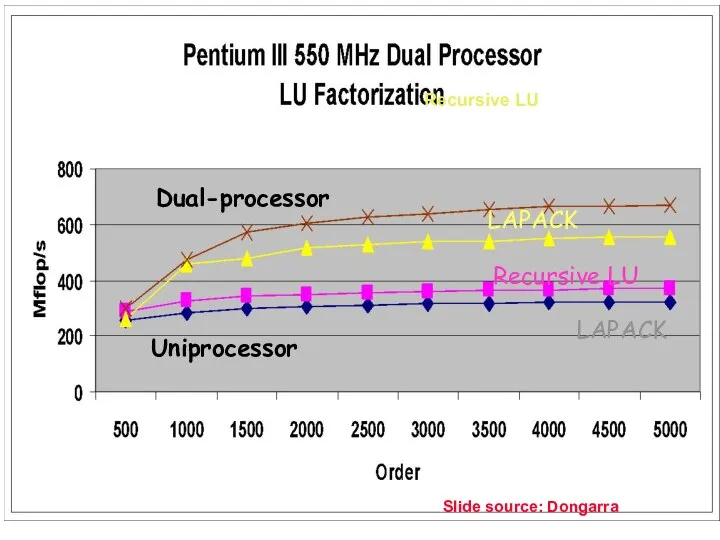
LAPACK
Recursive LU
Recursive LU
LAPACK
Dual-processor
Uniprocessor
Slide source: Dongarra
02/09/2006
CS267 Lecture 8
LAPACK
Recursive LU
Recursive LU
LAPACK
Dual-processor
Uniprocessor
Slide source: Dongarra
02/09/2006
CS267 Lecture 8
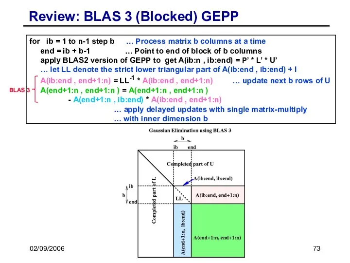
Review: BLAS 3 (Blocked) GEPP
for ib = 1 to
02/09/2006
CS267 Lecture 8
Review: BLAS 3 (Blocked) GEPP
for ib = 1 to
02/09/2006
CS267 Lecture 8
Review: Row and Column Block Cyclic Layout
processors and matrix
02/09/2006
CS267 Lecture 8
Review: Row and Column Block Cyclic Layout
processors and matrix
02/09/2006
CS267 Lecture 8
Distributed GE with a 2D Block Cyclic Layout
block size
02/09/2006
CS267 Lecture 8
Distributed GE with a 2D Block Cyclic Layout
block size
02/09/2006
CS267 Lecture 8
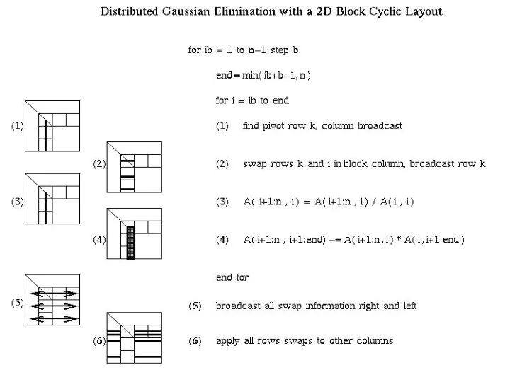
Distributed GE with a 2D Block Cyclic Layout
02/09/2006
CS267 Lecture 8
Distributed GE with a 2D Block Cyclic Layout
02/09/2006
CS267 Lecture 8
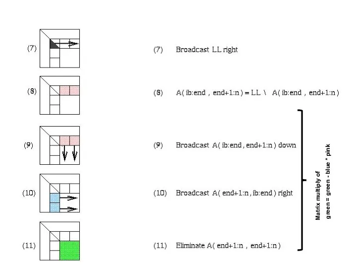
Matrix multiply of
green = green - blue *
02/09/2006
CS267 Lecture 8
Matrix multiply of
green = green - blue *
02/09/2006
CS267 Lecture 8
PDGESV = ScaLAPACK
parallel LU routine
Since it can
02/09/2006
CS267 Lecture 8
PDGESV = ScaLAPACK
parallel LU routine
Since it can
02/09/2006
CS267 Lecture 8
02/09/2006
CS267 Lecture 8
02/09/2006
CS267 Lecture 8
Scales well,
nearly full machine speed
02/09/2006
CS267 Lecture 8
Scales well,
nearly full machine speed
02/09/2006
CS267 Lecture 8
Old version,
pre 1998 Gordon Bell Prize
Still have ideas to
02/09/2006
CS267 Lecture 8
Old version,
pre 1998 Gordon Bell Prize
Still have ideas to
02/09/2006
CS267 Lecture 8
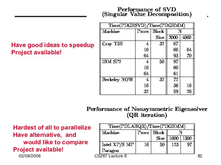
Have good ideas to speedup
Project available!
Hardest of all to
02/09/2006
CS267 Lecture 8
Have good ideas to speedup
Project available!
Hardest of all to
02/09/2006
CS267 Lecture 8
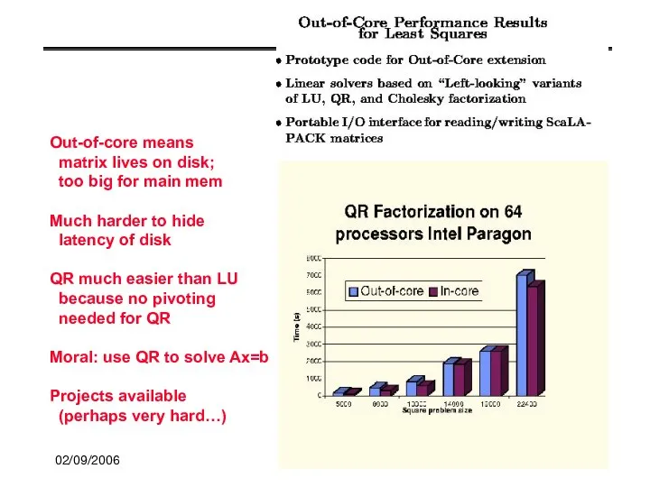
Out-of-core means
matrix lives on disk;
too big for
02/09/2006
CS267 Lecture 8
Out-of-core means
matrix lives on disk;
too big for
02/09/2006
CS267 Lecture 8
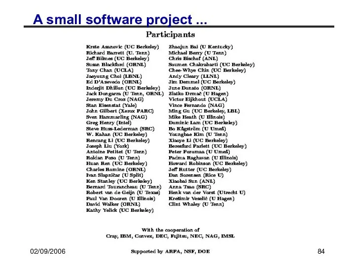
A small software project ...
02/09/2006
CS267 Lecture 8
A small software project ...
02/09/2006
CS267 Lecture 8
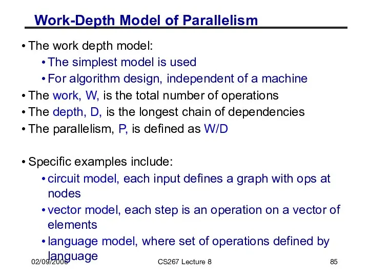
Work-Depth Model of Parallelism
The work depth model:
The simplest model
02/09/2006
CS267 Lecture 8
Work-Depth Model of Parallelism
The work depth model:
The simplest model
02/09/2006
CS267 Lecture 8
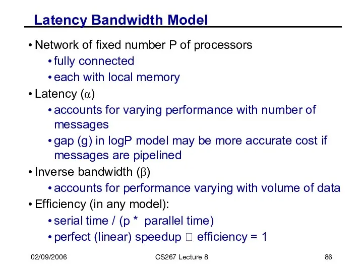
Latency Bandwidth Model
Network of fixed number P of processors
fully
02/09/2006
CS267 Lecture 8
Latency Bandwidth Model
Network of fixed number P of processors
fully
02/09/2006
CS267 Lecture 8
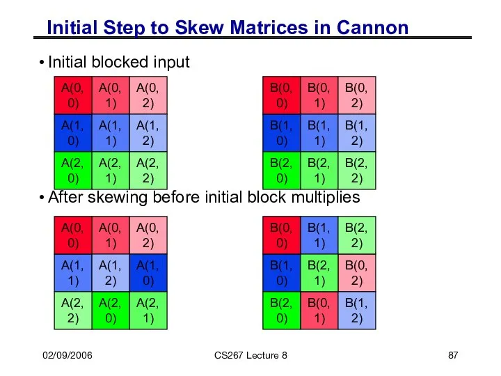
Initial Step to Skew Matrices in Cannon
Initial blocked input
After
02/09/2006
CS267 Lecture 8
Initial Step to Skew Matrices in Cannon
Initial blocked input
After
02/09/2006
CS267 Lecture 8
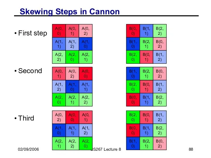
Skewing Steps in Cannon
First step
Second
Third
A(0,1)
A(0,2)
A(1,0)
A(2,0)
A(1,1)
A(1,2)
A(2,1)
A(2,2)
A(0,0)
B(0,1)
B(0,2)
B(1,0)
B(2,0)
B(1,1)
B(1,2)
B(2,1)
B(2,2)
B(0,0)
A(0,1)
A(0,2)
A(1,0)
A(2,0)
A(1,2)
A(2,1)
B(0,1)
B(0,2)
B(1,0)
B(2,0)
B(1,1)
B(1,2)
B(2,1)
B(2,2)
B(0,0)
A(0,1)
A(0,2)
A(1,0)
A(2,0)
A(1,1)
A(1,2)
A(2,1)
A(2,2)
A(0,0)
B(0,1)
B(0,2)
B(1,0)
B(2,0)
B(1,1)
B(1,2)
B(2,1)
B(2,2)
B(0,0)
A(1,1)
A(2,2)
A(0,0)
02/09/2006
CS267 Lecture 8
Skewing Steps in Cannon
First step
Second
Third
A(0,1)
A(0,2)
A(1,0)
A(2,0)
A(1,1)
A(1,2)
A(2,1)
A(2,2)
A(0,0)
B(0,1)
B(0,2)
B(1,0)
B(2,0)
B(1,1)
B(1,2)
B(2,1)
B(2,2)
B(0,0)
A(0,1)
A(0,2)
A(1,0)
A(2,0)
A(1,2)
A(2,1)
B(0,1)
B(0,2)
B(1,0)
B(2,0)
B(1,1)
B(1,2)
B(2,1)
B(2,2)
B(0,0)
A(0,1)
A(0,2)
A(1,0)
A(2,0)
A(1,1)
A(1,2)
A(2,1)
A(2,2)
A(0,0)
B(0,1)
B(0,2)
B(1,0)
B(2,0)
B(1,1)
B(1,2)
B(2,1)
B(2,2)
B(0,0)
A(1,1)
A(2,2)
A(0,0)
2/25/2009
CS267 Lecture 8
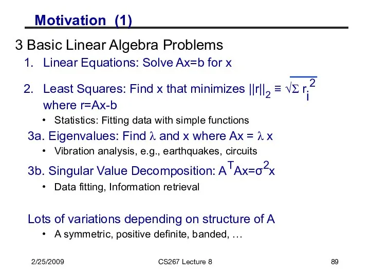
Motivation (1)
3 Basic Linear Algebra Problems
Linear Equations: Solve Ax=b
2/25/2009
CS267 Lecture 8
Motivation (1)
3 Basic Linear Algebra Problems
Linear Equations: Solve Ax=b
2/25/2009
CS267 Lecture 8
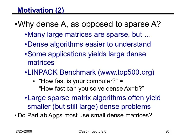
Motivation (2)
Why dense A, as opposed to sparse
2/25/2009
CS267 Lecture 8
Motivation (2)
Why dense A, as opposed to sparse
02/25/2009
CS267 Lecture 8
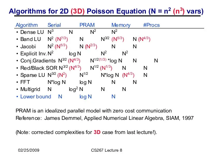
Algorithms for 2D (3D) Poisson Equation (N = n2
02/25/2009
CS267 Lecture 8
Algorithms for 2D (3D) Poisson Equation (N = n2
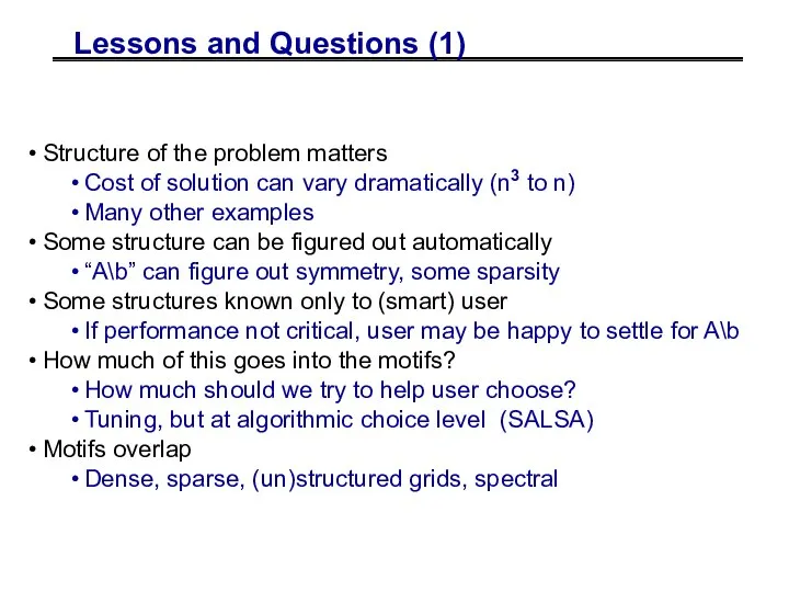
Lessons and Questions (1)
Structure of the problem matters
Cost of solution can
Lessons and Questions (1)
Structure of the problem matters
Cost of solution can
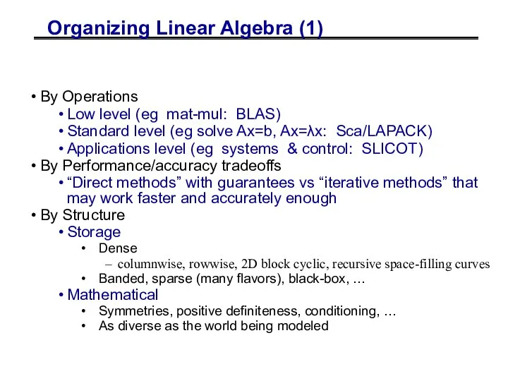
Organizing Linear Algebra (1)
By Operations
Low level (eg mat-mul: BLAS)
Standard level (eg
Organizing Linear Algebra (1)
By Operations
Low level (eg mat-mul: BLAS)
Standard level (eg
Organizing Linear Algebra (2)
By Data Type
Real vs Complex
Floating point (fixed or
Organizing Linear Algebra (2)
By Data Type
Real vs Complex
Floating point (fixed or
For all linear algebra problems:
Ex: LAPACK Table of Contents
Linear Systems
Least Squares
Overdetermined,
For all linear algebra problems:
Ex: LAPACK Table of Contents
Linear Systems
Least Squares
Overdetermined,
For all matrix/problem structures:
Ex: LAPACK Table of Contents
BD – bidiagonal
GB –
For all matrix/problem structures:
Ex: LAPACK Table of Contents
BD – bidiagonal
GB –
For all matrix/problem structures:
Ex: LAPACK Table of Contents
BD – bidiagonal
GB –
For all matrix/problem structures:
Ex: LAPACK Table of Contents
BD – bidiagonal
GB –
For all matrix/problem structures:
Ex: LAPACK Table of Contents
BD – bidiagonal
GB –
For all matrix/problem structures:
Ex: LAPACK Table of Contents
BD – bidiagonal
GB –
For all matrix/problem structures:
Ex: LAPACK Table of Contents
BD – bidiagonal
GB –
For all matrix/problem structures:
Ex: LAPACK Table of Contents
BD – bidiagonal
GB –
For all matrix/problem structures:
Ex: LAPACK Table of Contents
BD – bidiagonal
GB –
For all matrix/problem structures:
Ex: LAPACK Table of Contents
BD – bidiagonal
GB –
For all matrix/problem structures:
Ex: LAPACK Table of Contents
BD – bidiagonal
GB –
For all matrix/problem structures:
Ex: LAPACK Table of Contents
BD – bidiagonal
GB –
For all matrix/problem structures:
Ex: LAPACK Table of Contents
BD – bidiagonal
GB –
For all matrix/problem structures:
Ex: LAPACK Table of Contents
BD – bidiagonal
GB –
For all data types:
Ex: LAPACK Table of Contents
Real and complex
Single and
For all data types:
Ex: LAPACK Table of Contents
Real and complex
Single and
Organizing Linear Algebra (3)
www.netlib.org/lapack
www.netlib.org/scalapack
www.cs.utk.edu/~dongarra/etemplates
www.netlib.org/templates
gams.nist.gov
Organizing Linear Algebra (3)
www.netlib.org/lapack
www.netlib.org/scalapack
www.cs.utk.edu/~dongarra/etemplates
www.netlib.org/templates
gams.nist.gov
 Математический паркет
 Точки, прямые, отрезки. Задания для устного счета. Упражнение 1
 Показательные уравнения
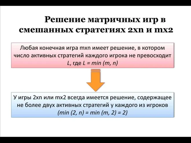 Решение матричных игр в смешанных стратегиях 2xn и mx2
 Статистические критерии в спортивной метрологии
 Тригонометрические уравнения
 Объём шара
 Презентация по математике "Нейтронная обработка драгоценных и полудрагоценных камней для ювелирной промышленности" - скачат
 Квадратные уравнения. Обобщающий урок
 Разложение квадратного трёхчлена на множители
 «Модуль» Элективный курс в рамках предпрофильной подготовки учащихся 9-х классов по математике Подготовила: Епанчинцева Г.
 Путешествие смешариков в стране математики (интерактивная игра)
 Табличное умножение. Выполнили: Иудкина Маша, Лесонен Настя, Силина Надя.
 Основные показатели ремонтопригодности
 Многогранники
 График квадратичной функции
 Прямокутник. Його властивості та ознаки. (8 класс)
 Решение примеров в пределах 10
 События. 5 класс. Учебник Зубаревой
 Математикалық ойын
 Тригонометрические уравнения
 Қысқаша көбейту формулалары
 Формулы для нахождения площади треугольника
 Принцип неопределенности Гейзенберга
 Математическая логика. (Тема 2)
 The quadrangle
 Модуль «Алгебра» №12
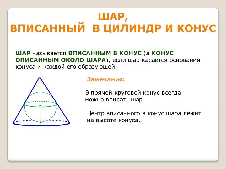 Шар, вписанный в цилиндр и конус