- Forecasting with bayesian techniques MP

Содержание
- 2. Lecture Objectives Introduce the idea of and rationale for Bayesian perspective and Bayesian VARs Understand the
- 3. Introduction: Two Perspectives in Econometrics Let θ be a vector of parameters to be estimated using
- 4. Outline Why a Bayesian Approach to VARs? Brief Introduction to Bayesian Econometrics Analytical Examples Estimating a
- 5. Why a Bayesian Approach to VAR? Dimensionality problem with VARs: y contains n variables, p lags
- 6. Usually, only a fraction of estimated coefficients are statistically significant parsimonious modeling should be favored What
- 7. Combining information: prior and posterior Bayesian coefficient estimates combine information in the prior with evidence from
- 8. Shrinkage There are many approaches to reducing over-parameterization in VARs A common idea is shrinkage Incorporating
- 9. Forecasting Performance of BVAR vs. alternatives Source: Litterman, 1986 BVAR provides better forecast of Real GNP
- 10. Introduction to Bayesian Econometrics: Objects of Interest Objects of interest: Prior distribution: Likelihood function: - likelihood
- 11. Bayesian Econometrics: Objects of Interest (2) The marginal likelihood… …is independent of the parameters of the
- 12. Bayesian Econometrics: maximizing criterion For practical purposes, it is useful to focus on the criterion: Traditionally,
- 13. Bayesian Econometrics : maximizing criterion (2) Maximizing C(θ) gives the Bayes mode. In some cases (i.e.
- 14. Analytical Examples Let’s work on some analytical examples: Sample mean Linear regression model
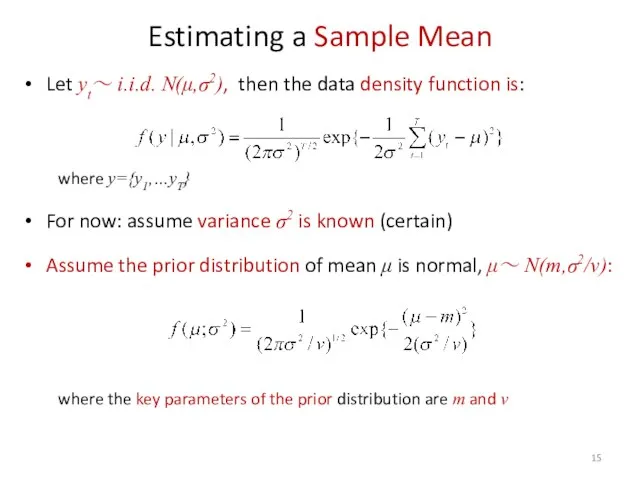
- 15. Estimating a Sample Mean Let yt~ i.i.d. N(μ,σ2), then the data density function is: where y={y1,…yT}
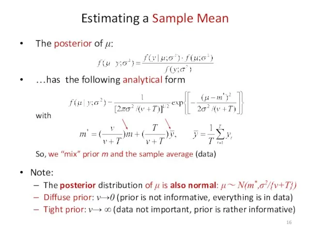
- 16. Estimating a Sample Mean The posterior of μ: …has the following analytical form with So, we
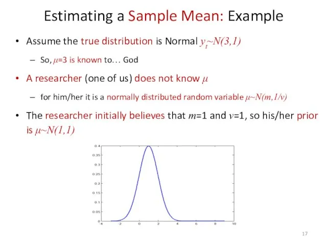
- 17. Estimating a Sample Mean: Example Assume the true distribution is Normal yt~N(3,1) So, μ=3 is known
- 18. Compute the posterior distribution as sample size increases Posterior with prior N(1,1) Already after 10 draws
- 19. Then, we look at more informative (tight) prior and set ν =50 (higher precision) Posterior with
- 20. Examples: Regression Model I Linear Regression model: where ut~ i.i.d. N(0,σ2) Assume: β is random and
- 21. Assume that the prior mean of β has multivariate Normal distribution N(m,σ2M): where the key parameters
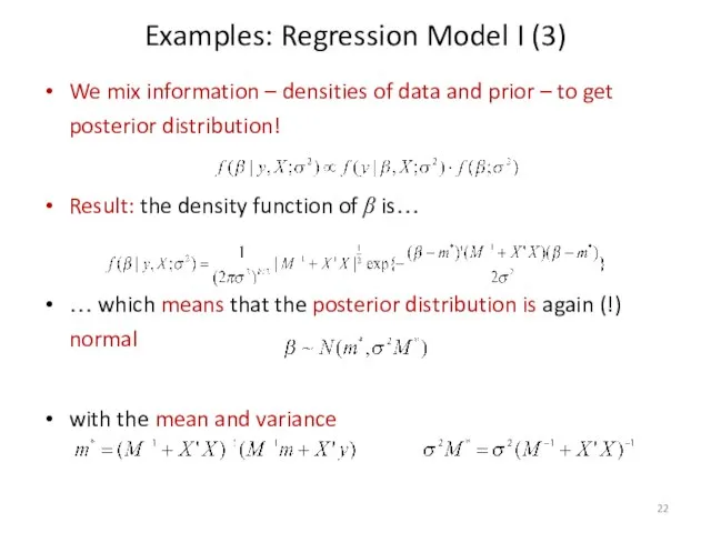
- 22. Examples: Regression Model I (3) We mix information – densities of data and prior – to
- 23. Since we do not like black boxes… there are 2 ways to get m* and M*
- 24. Define a “new” regression model We simply stack our “ingredients” together to mix the information (prior
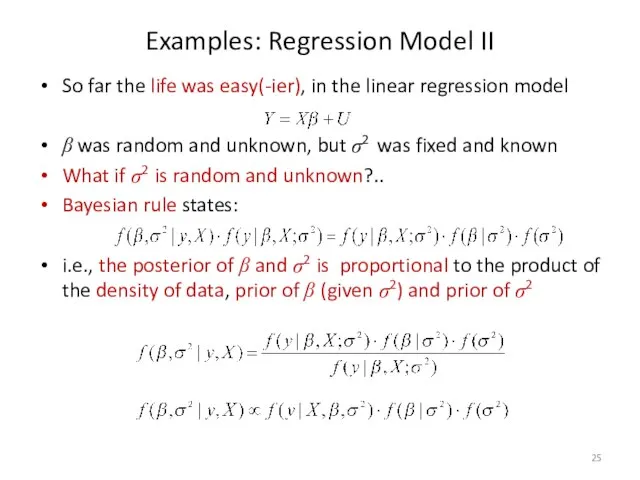
- 25. Examples: Regression Model II So far the life was easy(-ier), in the linear regression model β
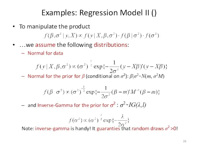
- 26. Examples: Regression Model II () To manipulate the product …we assume the following distributions: Normal for
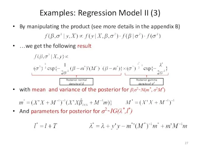
- 27. Examples: Regression Model II (3) By manipulating the product (see more details in the appendix B)
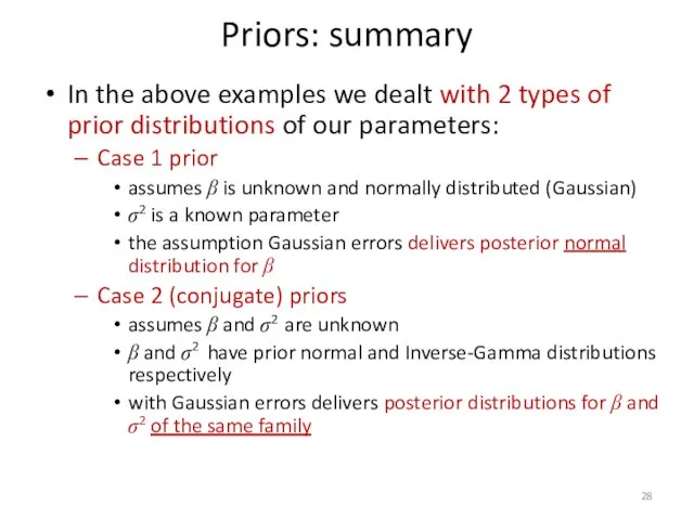
- 28. Priors: summary In the above examples we dealt with 2 types of prior distributions of our
- 29. Bayesian VARs Linear Regression examples will help us to deal with our main object – Bayesian
- 30. VAR in a matrix form: example Consider, as an example, a VAR for n variables and
- 31. How to Estimate a BVAR: Case 1 Prior Consider Case 1 prior for a VAR: coefficients
- 32. Before we see the case of an unknown Σe need to introduce a multivariate distribution to
- 33. How to Estimate a BVAR: Conjugate Priors Assume Conjugate priors: The VAR parameters A and Σe
- 34. BVARs: Minnesota Prior Implementation The Minnesota prior – a particular case of the “Case 1 prior”
- 35. The Minnesota prior The prior variance for the coefficient of lag k in equation i for
- 36. The Minnesota prior Interpretation: the prior on the first own lag is the prior on the
- 37. BVARs: Minnesota Prior Implementation
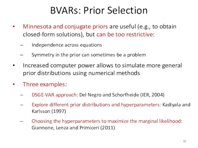
- 38. BVARs: Prior Selection Minnesota and conjugate priors are useful (e.g., to obtain closed-form solutions), but can
- 39. Del Negro and Schorfheide (2004): DSGE-VAR Approach Del Negro and Schorfheide (2004) We want to estimate
- 40. Del Negro and Schorfheide (2004) We estimate the following BVAR: The solution for the DSGE model
- 41. Del Negro and Schorfheide (2004) Parameter λ is a “weight” of “artificial” (prior) data from DSGE
- 42. Likelihood of the VAR of a DSGE Model Recall the likelihood function for an unconstrained VAR
- 43. Next step: we simulate s→∞ artificial observations (Y*,X*) from the DSGE …and replace sample moments like
- 44. Conditional on the parameters θ, the DSGE m+odel provides a conjugate priors for the BVAR For
- 45. DSGE-VAR posterior Posterior, conditional on θ : where Prior info, weighted by λT Information from Data
- 46. BVARs (under different λ’s) have advantage in forecasting performance (RMSE) vis-à-vis the unrestricted VAR The “optimal”
- 47. BVAR with the DSGE prior under the “optimal” λ has better forecasting performance than: the unrestricted
- 48. Kadiyala and Karlsson (1997) Small Model: a bivariate VAR with unemployment and industrial production Sample period:
- 49. Kadiyala and Karlsson (1997) Compare different priors based on the VAR forecasting performance (RMSE) Standard VAR(p)…
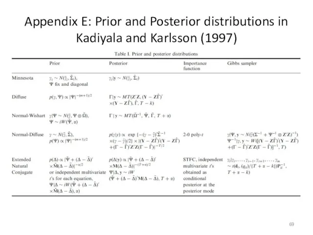
- 50. Prior distributions in K&K K&K use a number of competing prior distributions… Minnesota, Normal-Wishart, Normal-Diffuse, Extended
- 51. Prior distributions in K&K In the Small Model: For prior distributions, hyper-parameters π1= γ, π2=wγ are
- 52. Forecast Comparison in K&K: Small Model, unemployment Forecasting performance is markedly different for different priors Normal-Wishart,
- 53. Forecast Comparison in K&K: Large Model OLS and Diffuse priors produce worst forecasts in all cases
- 54. Giannone, Lenza and Primiceri (2011) Use three VARs to compare forecasting performance Small VAR: GDP, GDP
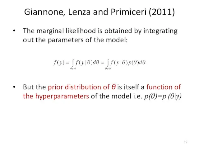
- 55. Giannone, Lenza and Primiceri (2011) The marginal likelihood is obtained by integrating out the parameters of
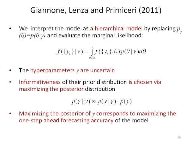
- 56. Giannone, Lenza and Primiceri (2011) We interpret the model as a hierarchical model by replacing pγ(θ)=p(θ|γ)
- 57. Giannone, Lenza and Primiceri (2011)
- 58. In all cases BVARs demonstrate better forecasting performance vis-à-vis the unrestricted VARs BVARs are roughly at
- 59. Conclusions BVARs is a useful tool to improve forecasts This is not a “black box” posterior
- 60. Thank You!
- 61. Appendix A: Remarks about the marginal likelihood Remarks about the marginal likelihood: If we have M1,….MN
- 62. Appendix A: Remarks about the marginal likelihood Remarks about the marginal likelihood: Predict the first observation
- 63. Appendix B: Linear Regression with conjugate priors To calculate the posterior distribution for parameters …we assume
- 64. Rearranging the expressions under the exponents we have the following: where Further denote … and rewrite
- 65. Therefore we have Normal posterior distribution for β: β|σ2 ̴ N(m*, σ2M*) And Invesrse Gamma posterior
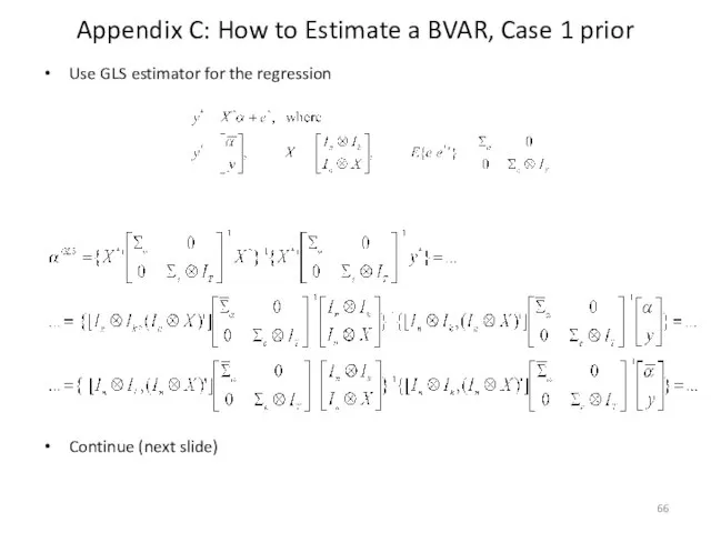
- 66. Appendix C: How to Estimate a BVAR, Case 1 prior Use GLS estimator for the regression
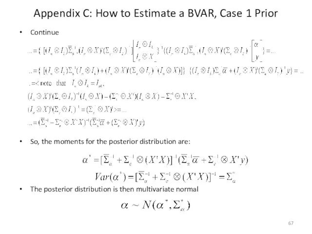
- 67. Appendix C: How to Estimate a BVAR, Case 1 Prior Continue So, the moments for the
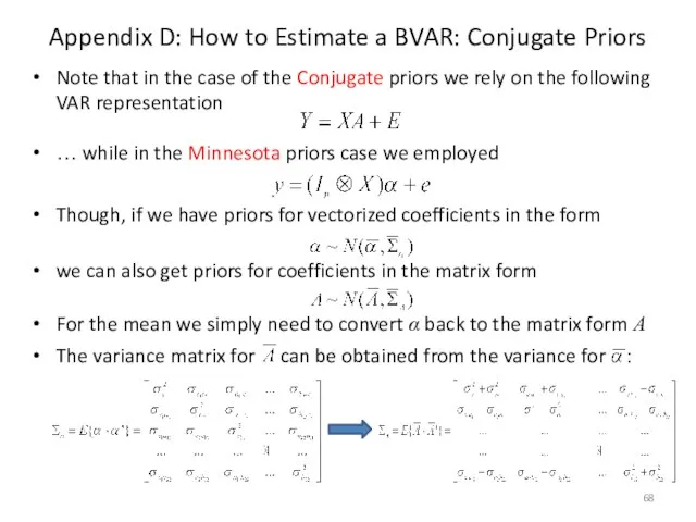
- 68. Appendix D: How to Estimate a BVAR: Conjugate Priors Note that in the case of the
- 69. Appendix E: Prior and Posterior distributions in Kadiyala and Karlsson (1997)
- 70. Appendix E: Posterior distributions of forecast for unemployment and industrial production in K&K (1997), h=4, T0
- 71. Appendix E: Posterior distribution of the unemployment rate forecast in K&K (1997)
- 73. Скачать презентацию
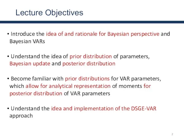
Lecture Objectives
Introduce the idea of and rationale for Bayesian perspective
Lecture Objectives
Introduce the idea of and rationale for Bayesian perspective
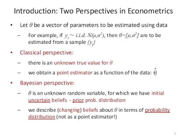
Introduction: Two Perspectives in Econometrics
Let θ be a vector of parameters
Introduction: Two Perspectives in Econometrics
Let θ be a vector of parameters

Outline
Why a Bayesian Approach to VARs?
Brief Introduction to Bayesian Econometrics
Analytical Examples
Estimating
Outline
Why a Bayesian Approach to VARs?
Brief Introduction to Bayesian Econometrics
Analytical Examples
Estimating
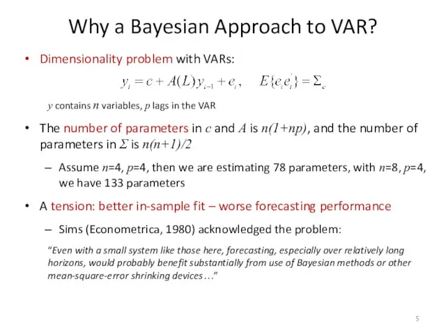
Why a Bayesian Approach to VAR?
Dimensionality problem with VARs:
y contains
Why a Bayesian Approach to VAR?
Dimensionality problem with VARs:
y contains
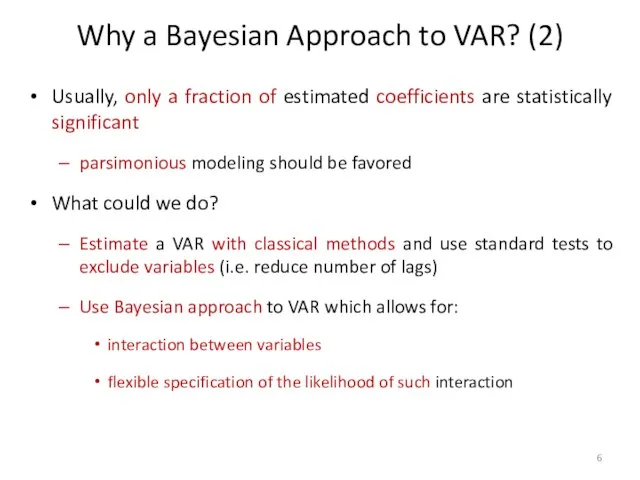
Usually, only a fraction of estimated coefficients are statistically significant
parsimonious modeling
Usually, only a fraction of estimated coefficients are statistically significant
parsimonious modeling
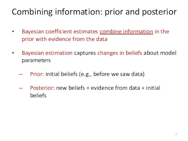
Combining information: prior and posterior
Bayesian coefficient estimates combine information in the
Combining information: prior and posterior
Bayesian coefficient estimates combine information in the
Shrinkage
There are many approaches to reducing over-parameterization in VARs
A common idea
Shrinkage
There are many approaches to reducing over-parameterization in VARs
A common idea
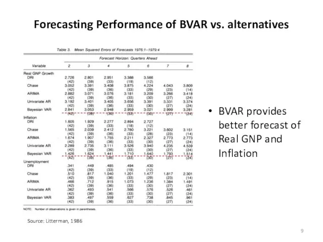
Forecasting Performance of BVAR vs. alternatives
Source: Litterman, 1986
BVAR provides better forecast
Forecasting Performance of BVAR vs. alternatives
Source: Litterman, 1986
BVAR provides better forecast
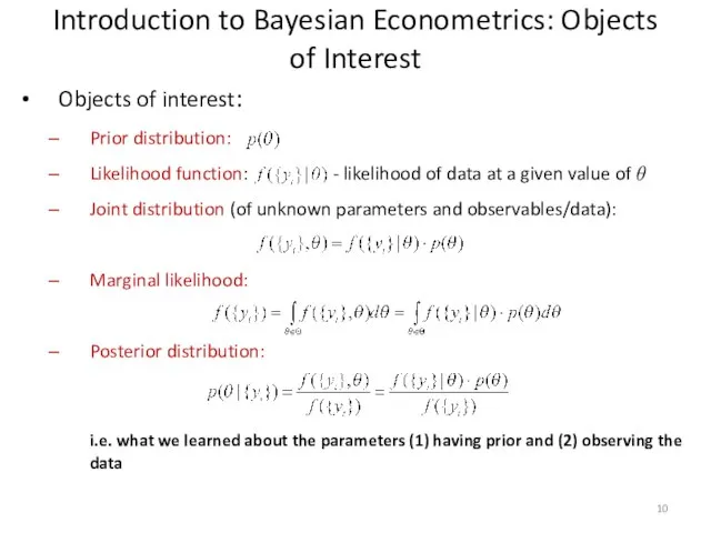
Introduction to Bayesian Econometrics: Objects of Interest
Objects of interest:
Prior distribution:
Likelihood function:
Introduction to Bayesian Econometrics: Objects of Interest
Objects of interest:
Prior distribution:
Likelihood function:
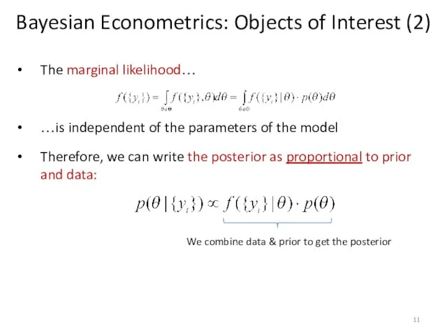
Bayesian Econometrics: Objects of Interest (2)
The marginal likelihood…
…is independent of
Bayesian Econometrics: Objects of Interest (2)
The marginal likelihood…
…is independent of
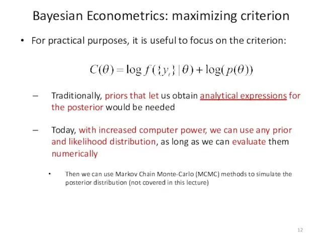
Bayesian Econometrics: maximizing criterion
For practical purposes, it is useful to focus
Bayesian Econometrics: maximizing criterion
For practical purposes, it is useful to focus
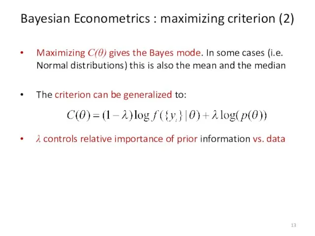
Bayesian Econometrics : maximizing criterion (2)
Maximizing C(θ) gives the Bayes mode.
Bayesian Econometrics : maximizing criterion (2)
Maximizing C(θ) gives the Bayes mode.
Analytical Examples
Let’s work on some analytical examples:
Sample mean
Linear regression model
Analytical Examples
Let’s work on some analytical examples:
Sample mean
Linear regression model
Estimating a Sample Mean
Let yt~ i.i.d. N(μ,σ2), then the data density
Estimating a Sample Mean
Let yt~ i.i.d. N(μ,σ2), then the data density
Estimating a Sample Mean
The posterior of μ:
…has the following analytical form
Estimating a Sample Mean
The posterior of μ:
…has the following analytical form
Estimating a Sample Mean: Example
Assume the true distribution is Normal yt~N(3,1)
So,
Estimating a Sample Mean: Example
Assume the true distribution is Normal yt~N(3,1)
So,
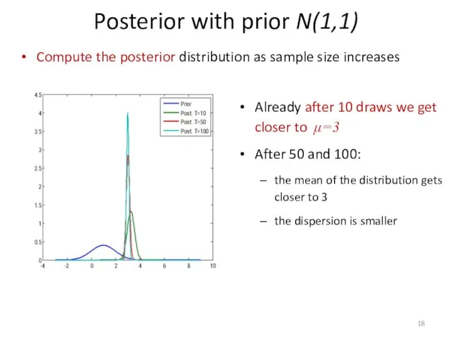
Compute the posterior distribution as sample size increases
Posterior with prior N(1,1)
Already
Compute the posterior distribution as sample size increases
Posterior with prior N(1,1)
Already
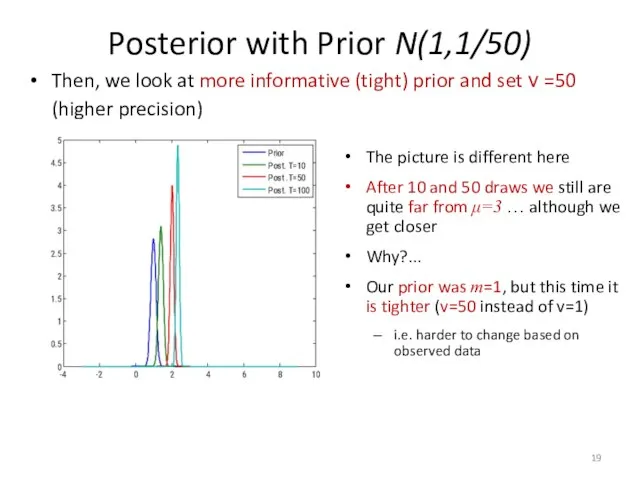
Then, we look at more informative (tight) prior and set ν
Then, we look at more informative (tight) prior and set ν

Examples: Regression Model I
Linear Regression model:
where ut~ i.i.d. N(0,σ2)
Assume:
β is
Examples: Regression Model I
Linear Regression model:
where ut~ i.i.d. N(0,σ2)
Assume:
β is
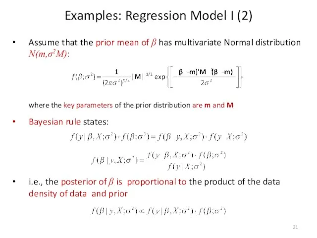
Assume that the prior mean of β has multivariate Normal distribution
Assume that the prior mean of β has multivariate Normal distribution
Examples: Regression Model I (3)
We mix information – densities of data
Examples: Regression Model I (3)
We mix information – densities of data
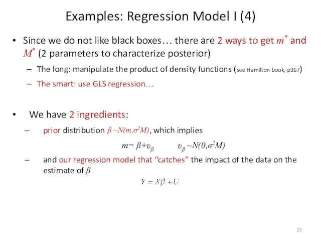
Since we do not like black boxes… there are 2 ways
Since we do not like black boxes… there are 2 ways
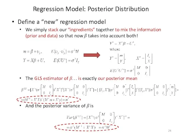
Define a “new” regression model
We simply stack our “ingredients” together to
Define a “new” regression model
We simply stack our “ingredients” together to
Examples: Regression Model II
So far the life was easy(-ier), in the
Examples: Regression Model II
So far the life was easy(-ier), in the
Examples: Regression Model II ()
To manipulate the product
…we assume the
Examples: Regression Model II ()
To manipulate the product
…we assume the
Examples: Regression Model II (3)
By manipulating the product (see more details
Examples: Regression Model II (3)
By manipulating the product (see more details
Priors: summary
In the above examples we dealt with 2 types
Priors: summary
In the above examples we dealt with 2 types
Bayesian VARs
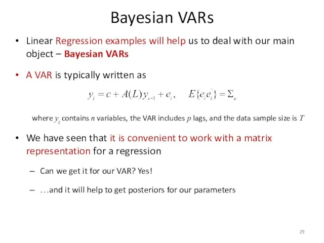
Linear Regression examples will help us to deal with our
Bayesian VARs
Linear Regression examples will help us to deal with our
VAR in a matrix form: example
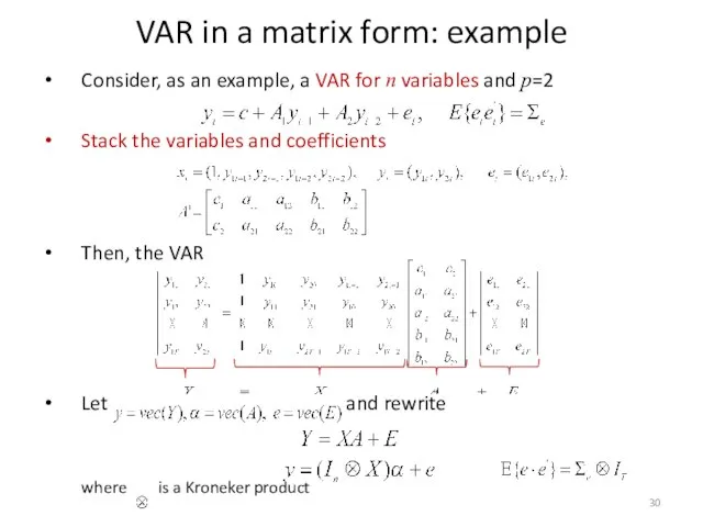
Consider, as an example, a VAR
VAR in a matrix form: example
Consider, as an example, a VAR

How to Estimate a BVAR: Case 1 Prior
Consider Case 1 prior
How to Estimate a BVAR: Case 1 Prior
Consider Case 1 prior
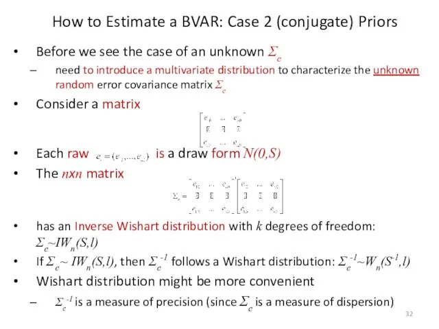
Before we see the case of an unknown Σe
need to introduce
Before we see the case of an unknown Σe
need to introduce
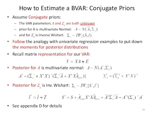
How to Estimate a BVAR: Conjugate Priors
Assume Conjugate priors:
The VAR parameters
How to Estimate a BVAR: Conjugate Priors
Assume Conjugate priors:
The VAR parameters
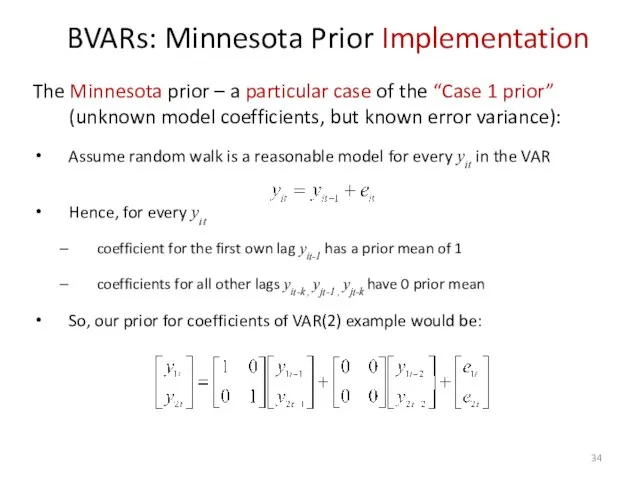
BVARs: Minnesota Prior Implementation
The Minnesota prior – a particular case of
BVARs: Minnesota Prior Implementation
The Minnesota prior – a particular case of

The Minnesota prior
The prior variance for the coefficient of lag k
The Minnesota prior
The prior variance for the coefficient of lag k
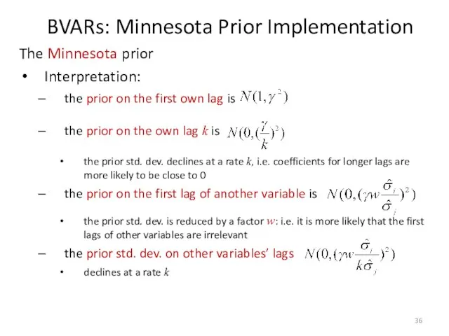
The Minnesota prior
Interpretation:
the prior on the first own lag is
The Minnesota prior
Interpretation:
the prior on the first own lag is
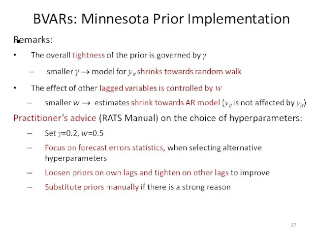
BVARs: Minnesota Prior Implementation
BVARs: Minnesota Prior Implementation
BVARs: Prior Selection
Minnesota and conjugate priors are useful (e.g., to obtain
BVARs: Prior Selection
Minnesota and conjugate priors are useful (e.g., to obtain
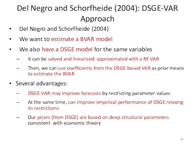
Del Negro and Schorfheide (2004): DSGE-VAR Approach
Del Negro and Schorfheide (2004)
We
Del Negro and Schorfheide (2004): DSGE-VAR Approach
Del Negro and Schorfheide (2004)
We
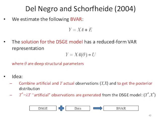
Del Negro and Schorfheide (2004)
We estimate the following BVAR:
The solution for
Del Negro and Schorfheide (2004)
We estimate the following BVAR:
The solution for
Del Negro and Schorfheide (2004)
Parameter λ is a “weight” of “artificial”
Del Negro and Schorfheide (2004)
Parameter λ is a “weight” of “artificial”
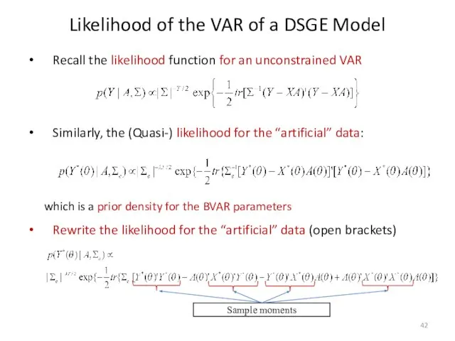
Likelihood of the VAR of a DSGE Model
Recall the likelihood function
Likelihood of the VAR of a DSGE Model
Recall the likelihood function
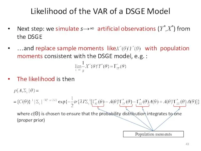
Next step: we simulate s→∞ artificial observations (Y*,X*) from the DSGE
…and
Next step: we simulate s→∞ artificial observations (Y*,X*) from the DSGE
…and
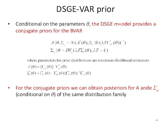
Conditional on the parameters θ, the DSGE m+odel provides a conjugate
Conditional on the parameters θ, the DSGE m+odel provides a conjugate

DSGE-VAR posterior
Posterior, conditional on θ :
where
Prior info, weighted by λT
Information from
DSGE-VAR posterior
Posterior, conditional on θ :
where
Prior info, weighted by λT
Information from
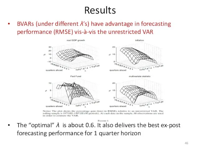
BVARs (under different λ’s) have advantage in forecasting performance (RMSE) vis-à-vis
BVARs (under different λ’s) have advantage in forecasting performance (RMSE) vis-à-vis
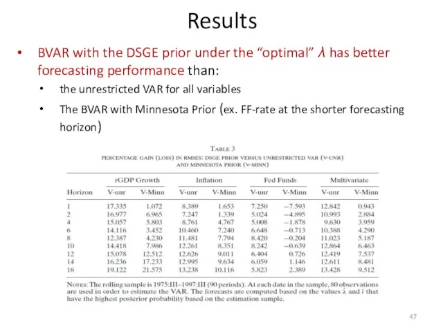
BVAR with the DSGE prior under the “optimal” λ has better
BVAR with the DSGE prior under the “optimal” λ has better
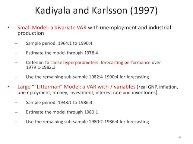
Kadiyala and Karlsson (1997)
Small Model: a bivariate VAR with unemployment and
Kadiyala and Karlsson (1997)
Small Model: a bivariate VAR with unemployment and
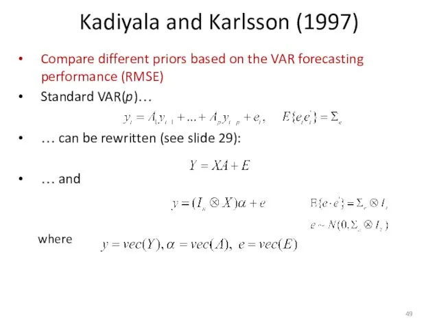
Kadiyala and Karlsson (1997)
Compare different priors based on the VAR forecasting
Kadiyala and Karlsson (1997)
Compare different priors based on the VAR forecasting
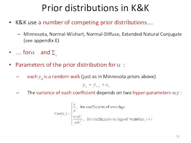
Prior distributions in K&K
K&K use a number of competing prior distributions…
Prior distributions in K&K
K&K use a number of competing prior distributions…
Prior distributions in K&K
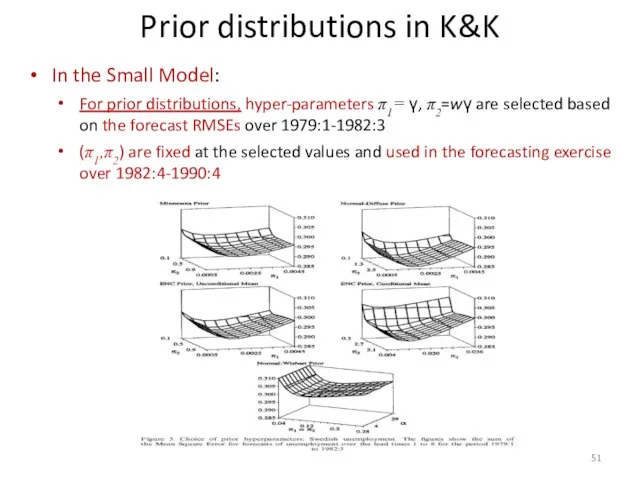
In the Small Model:
For prior distributions, hyper-parameters π1=
Prior distributions in K&K
In the Small Model:
For prior distributions, hyper-parameters π1=
Forecast Comparison in K&K: Small Model, unemployment
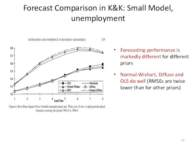
Forecasting performance is markedly
Forecast Comparison in K&K: Small Model, unemployment
Forecasting performance is markedly
Forecast Comparison in K&K: Large Model
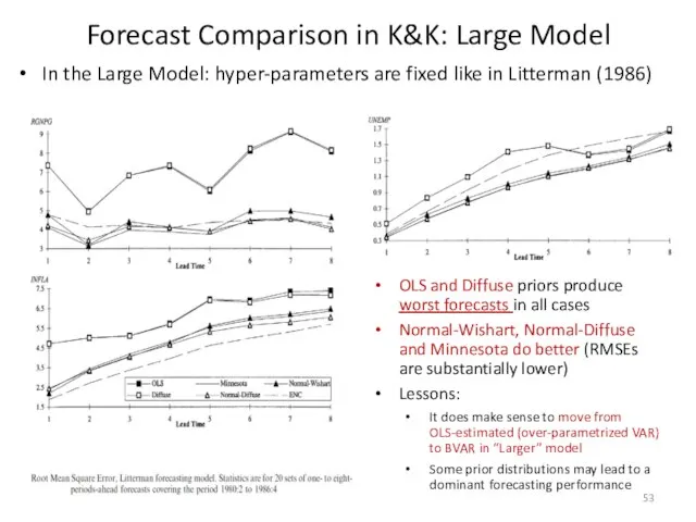
OLS and Diffuse priors produce worst
Forecast Comparison in K&K: Large Model
OLS and Diffuse priors produce worst
Giannone, Lenza and Primiceri (2011)
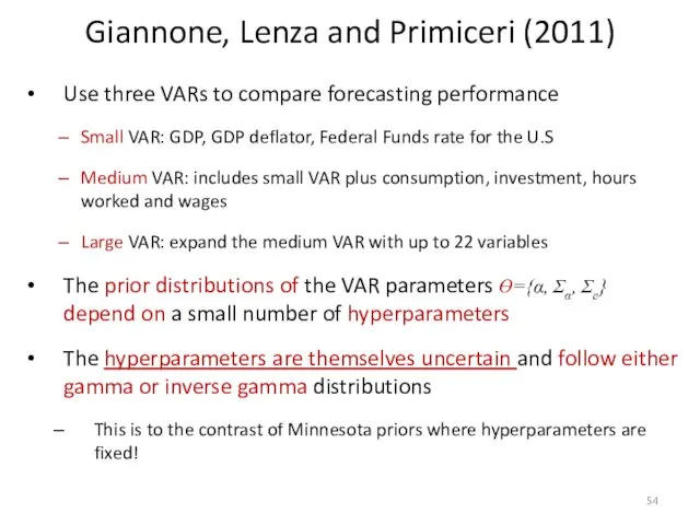
Use three VARs to compare forecasting performance
Small
Giannone, Lenza and Primiceri (2011)
Use three VARs to compare forecasting performance
Small
Giannone, Lenza and Primiceri (2011)
The marginal likelihood is obtained by integrating
Giannone, Lenza and Primiceri (2011)
The marginal likelihood is obtained by integrating
Giannone, Lenza and Primiceri (2011)
We interpret the model as a hierarchical
Giannone, Lenza and Primiceri (2011)
We interpret the model as a hierarchical
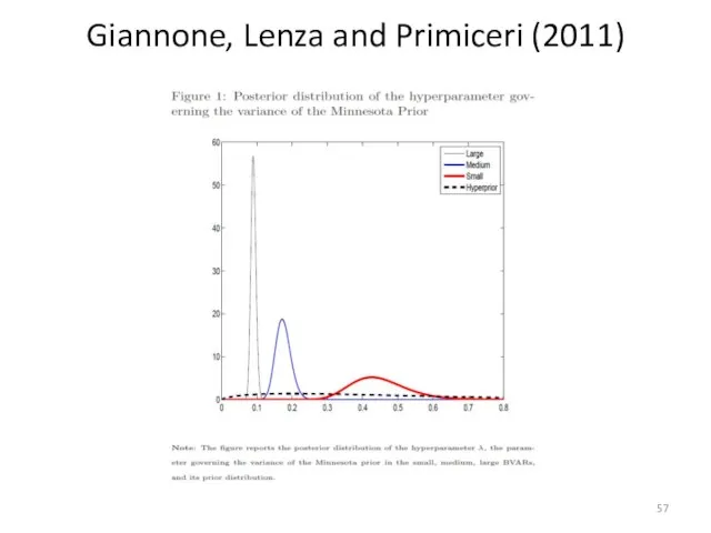
Giannone, Lenza and Primiceri (2011)
Giannone, Lenza and Primiceri (2011)
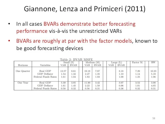
In all cases BVARs demonstrate better forecasting performance vis-à-vis the unrestricted
In all cases BVARs demonstrate better forecasting performance vis-à-vis the unrestricted

Conclusions
BVARs is a useful tool to improve forecasts
This is not a
Conclusions
BVARs is a useful tool to improve forecasts
This is not a

Thank You!
Thank You!
Appendix A: Remarks about the marginal likelihood
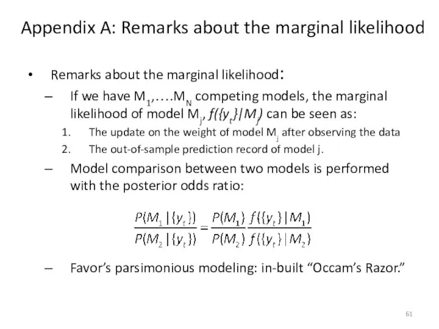
Remarks about the marginal likelihood:
If
Appendix A: Remarks about the marginal likelihood
Remarks about the marginal likelihood:
If
Appendix A: Remarks about the marginal likelihood
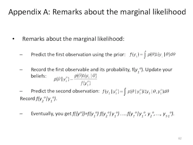
Remarks about the marginal likelihood:
Predict
Appendix A: Remarks about the marginal likelihood
Remarks about the marginal likelihood:
Predict
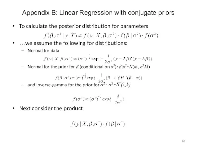
Appendix B: Linear Regression with conjugate priors
To calculate the posterior distribution
Appendix B: Linear Regression with conjugate priors
To calculate the posterior distribution
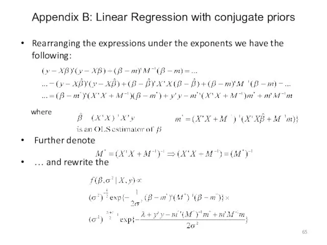
Rearranging the expressions under the exponents we have the following:
where
Rearranging the expressions under the exponents we have the following:
where
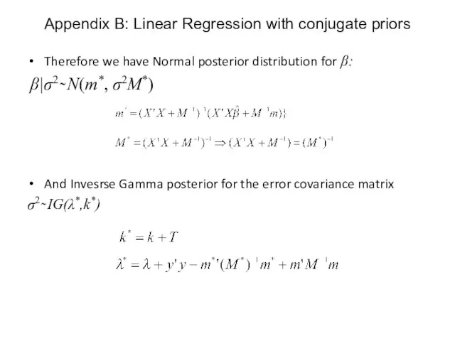
Therefore we have Normal posterior distribution for β:
β|σ2 ̴ N(m*,
Therefore we have Normal posterior distribution for β:
β|σ2 ̴ N(m*,
Appendix C: How to Estimate a BVAR, Case 1 prior
Use GLS
Appendix C: How to Estimate a BVAR, Case 1 prior
Use GLS
Appendix C: How to Estimate a BVAR, Case 1 Prior
Continue
So, the
Appendix C: How to Estimate a BVAR, Case 1 Prior
Continue
So, the
Appendix D: How to Estimate a BVAR: Conjugate Priors
Note that in
Appendix D: How to Estimate a BVAR: Conjugate Priors
Note that in
Appendix E: Prior and Posterior distributions in Kadiyala and Karlsson (1997)
Appendix E: Prior and Posterior distributions in Kadiyala and Karlsson (1997)
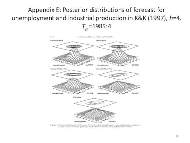
Appendix E: Posterior distributions of forecast for unemployment and industrial production
Appendix E: Posterior distributions of forecast for unemployment and industrial production
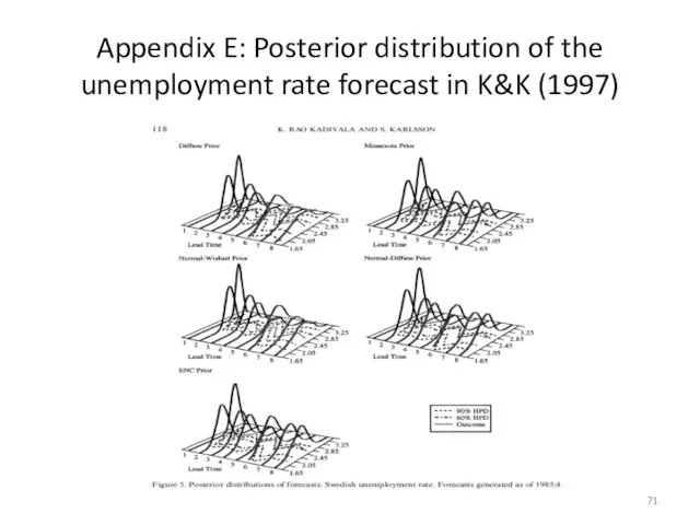
Appendix E: Posterior distribution of the unemployment rate forecast in K&K
Appendix E: Posterior distribution of the unemployment rate forecast in K&K
 Упрощение выражений. 5 класс
 Обыкновенные дроби. Игра "Счастливый случай"
 Математические основы построения экспертной модели при расплывчатости границ между смежными рангами пожара
 Мультимедийное пособие «Функция»
 Исторические комбинаторные задачи. 6 - 8 классы
 Математика XIX ст. Жан Батист Жозеф Фур'є
 Теорема Пифагора
 Понятие модели. Способы представления моделей. (Лекция 4)
 Состав чисел в приделах 10. Закрепление
 Площадь и объем
 Сочетания. Формирование умений и навыков
 Равные выражения. Сравниваем выражения
 Угол между векторами. Скалярное произведение векторов
 Задачи на вероятность
 Примеры решения комбинаторных задач Примеры решения комбинаторных задач
  Функция y = x2 и её график
 Призма
 Преобразование графика функции
 חשבון רוקחי 4 תרגילים+תשובות
 Различные способы решения систем двух линейных уравнений с двумя переменными
 Угол между плоскостями
 Число и цифра 4
 Деление обыкновенных дробей Математика, 6 класс
 Математика 4 класс Морозова Валентина Анатольевна учитель начальных классов МОУ Шевыряловская основная общеобразовательная шк
 Прямая. Отрезок. Луч
 Интерактивные тренинги по математике для подготовки к ЕГЭ
 Презентация на тему Сравнение предметов Математика 1 класс
 Презентация по математике "Юным умникам и умницам" - скачать