- Statistics. Data Description. Data Summarization. Numerical Measures of the Data

Содержание
- 2. Chapter Three: Numerical Measures of the Data Outline Introduction 3-1 Measures of Central Tendency 3-2 Measures
- 3. Chapter Three: Numerical Measures of the Data Objectives Summarize data using the measures of central tendency,
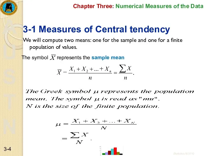
- 4. Chapter Three: Numerical Measures of the Data 3-1 Measures of Central tendency We will compute two
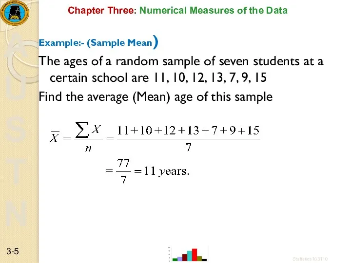
- 5. Chapter Three: Numerical Measures of the Data Example:- (Sample Mean) The ages of a random sample
- 6. Chapter Three: Numerical Measures of the Data Example:- population mean Statistics103110 3-
- 7. Chapter Three: Numerical Measures of the Data The Sample Mean for an Ungrouped Frequency Distribution Statistics103110
- 8. Chapter Three: Numerical Measures of the Data The Sample Mean for an Ungrouped Frequency Distribution –
- 9. Chapter Three: Numerical Measures of the Data The Sample Mean for a Grouped Frequency Distribution The
- 10. Important remark : In some situations the mean may not be representative of the data. As
- 11. Properties of the mean As stated, the mean is a widely used measure of central tendency
- 12. Chapter Three: Numerical Measures of the Data Median : The median splits the ordered data into
- 13. Chapter Three: Numerical Measures of the Data When there is an even number of values in
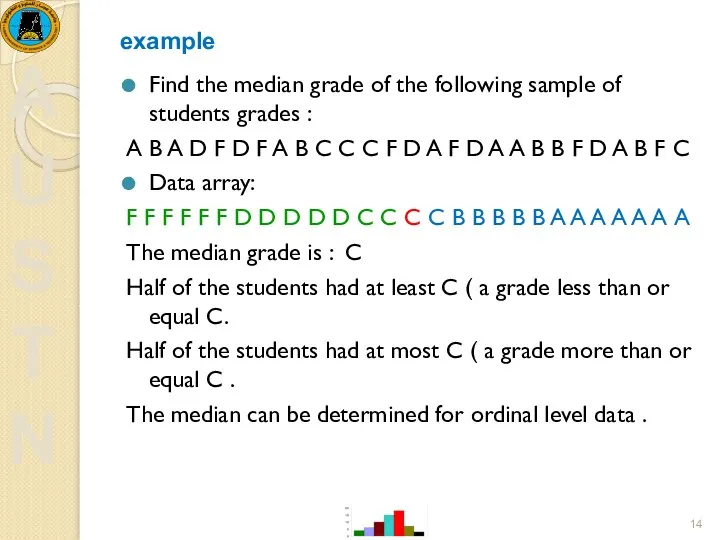
- 14. example Find the median grade of the following sample of students grades : A B A
- 15. Properties of the Median The major properties of the median are: The median is a unique
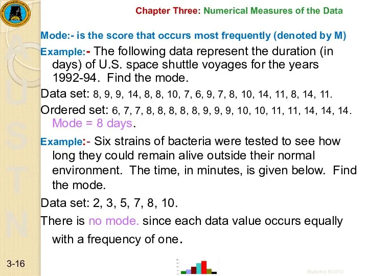
- 16. Chapter Three: Numerical Measures of the Data Mode:- is the score that occurs most frequently (denoted
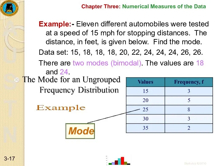
- 17. Chapter Three: Numerical Measures of the Data Example:- Eleven different automobiles were tested at a speed
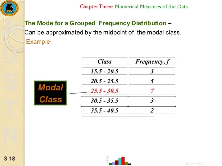
- 18. Chapter Three: Numerical Measures of the Data The Mode for a Grouped Frequency Distribution – Can
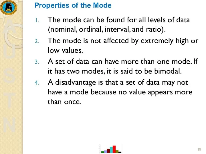
- 19. Properties of the Mode The mode can be found for all levels of data (nominal, ordinal,
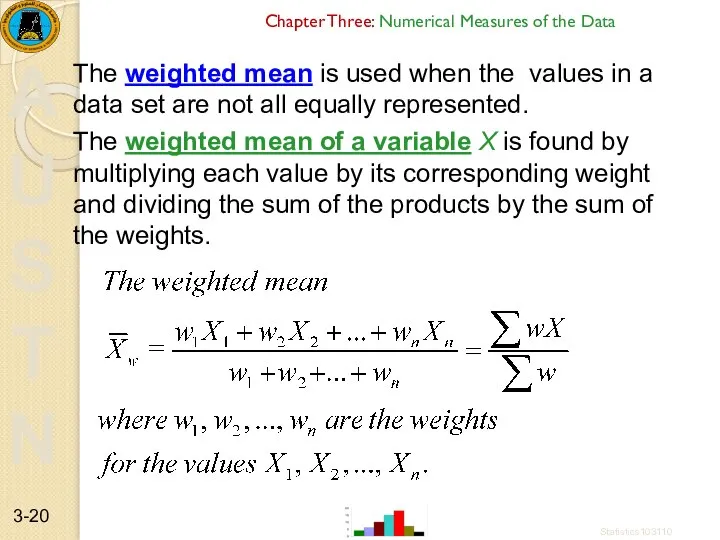
- 20. Chapter Three: Numerical Measures of the Data The weighted mean is used when the values in
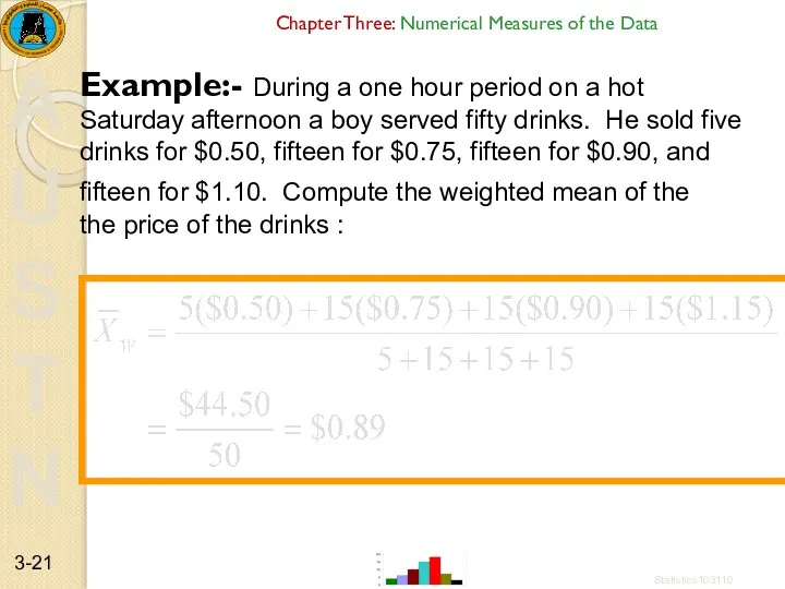
- 21. Chapter Three: Numerical Measures of the Data Example:- During a one hour period on a hot
- 22. Best measure of central tendency
- 23. Relationship between mean , median and mode and the shape of the distribution Symmetric – the
- 24. Chapter Three: Numerical Measures of the Data 3-2 Measures of Dispersion( variation) o the spread or
- 25. Variability -- provides a quantitative measure of the degree to which scores in a distribution are
- 26. Measures of dispersion are : The range , The interquartile range , The variance and standard
- 27. Example Compute the range of 6, 1, 2, 6, 11, 7, 3, 3 The largest value
- 28. The variance of a variable The variance is based on the deviation from the mean (
- 29. Chapter Three: Numerical Measures of the Data The population variance of a variable is the sum
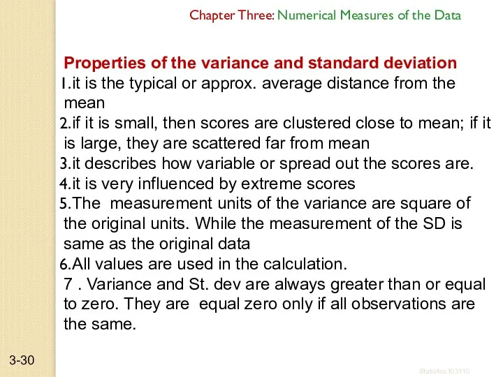
- 30. Properties of the variance and standard deviation it is the typical or approx. average distance from
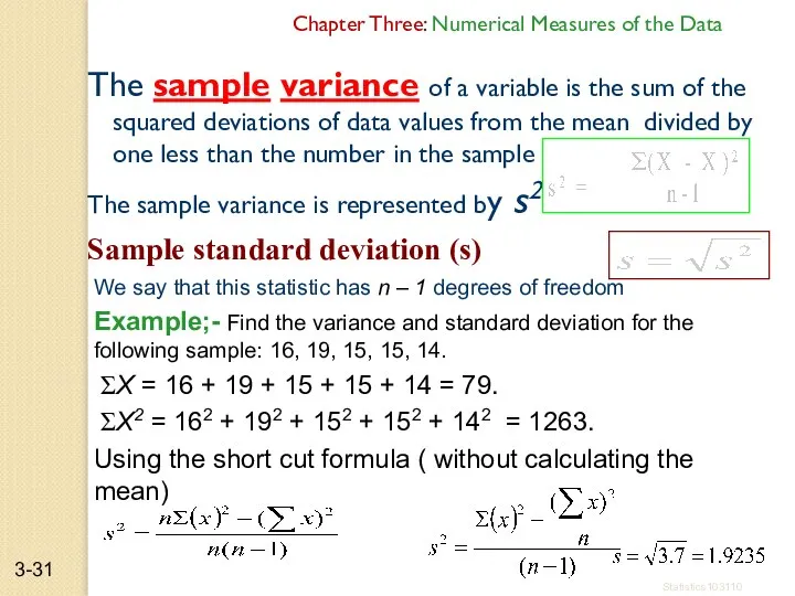
- 31. Chapter Three: Numerical Measures of the Data The sample variance of a variable is the sum
- 32. Symbols for Standard Deviation Sample Population σ σ x xσn Book Some graphics calculators Some non-graphics
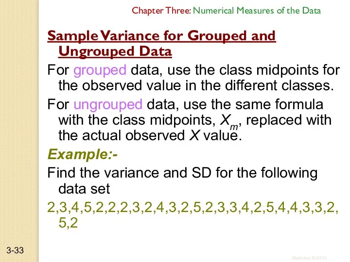
- 33. Chapter Three: Numerical Measures of the Data Sample Variance for Grouped and Ungrouped Data For grouped
- 34. Step one put the data I ungrouped frequency table Chapter Three: Numerical Measures of the Data
- 35. Example:- find the variance and SD for the frequency distribution of the data representing number of
- 36. Chapter Three: Numerical Measures of the Data Statistics103110 3-
- 37. Chapter Three: Numerical Measures of the Data Interpretation and Uses of the Standard Deviation The standard
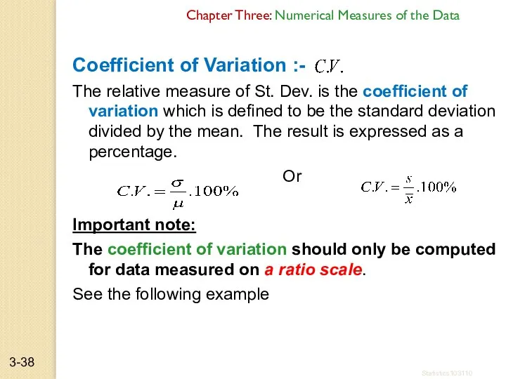
- 38. Chapter Three: Numerical Measures of the Data Coefficient of Variation :- The relative measure of St.
- 39. Example : To see why the coefficient of variation should not be applied to interval level
- 40. Advantages The coefficient of variation is useful because the standard deviation of data must always be
- 41. Example:- Data about the annual salary (000’s) and age of CEO’s in a number of firms
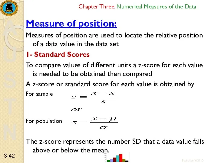
- 42. Chapter Three: Numerical Measures of the Data Measure of position: Measures of position are used to
- 43. Chapter Three: Numerical Measures of the Data Standard Scores (or z-scores) specify the exact location of
- 44. Chapter Three: Numerical Measures of the Data Characteristics of Standard Scores The shape of the distribution
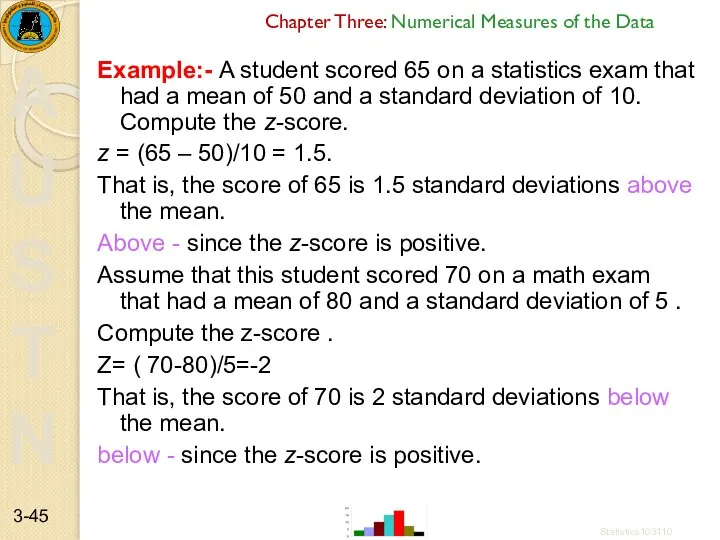
- 45. Chapter Three: Numerical Measures of the Data Example:- A student scored 65 on a statistics exam
- 46. Example:- a student scored 65 on a calculus test that had a mean of 50 and
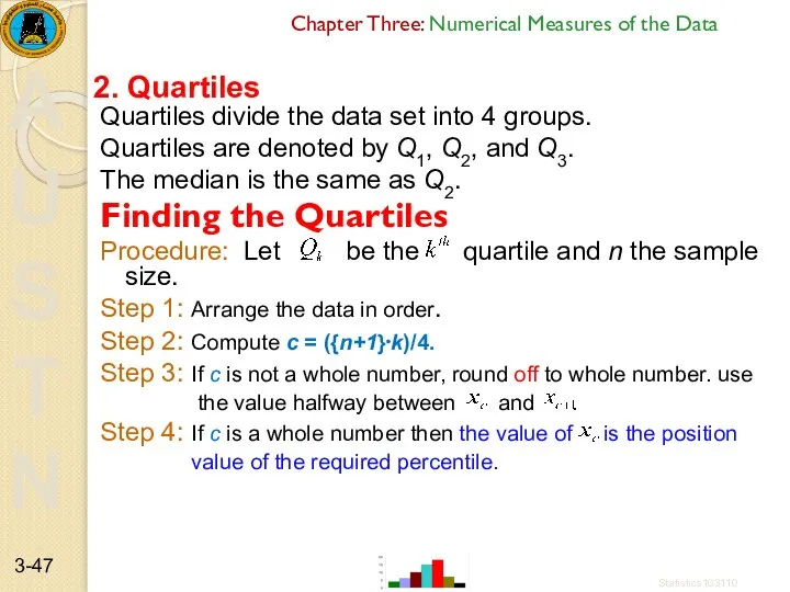
- 47. Chapter Three: Numerical Measures of the Data Quartiles divide the data set into 4 groups. Quartiles
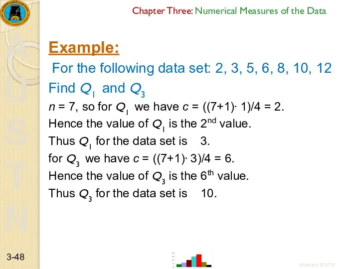
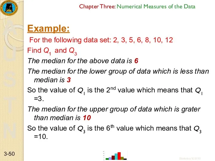
- 48. Chapter Three: Numerical Measures of the Data Example: For the following data set: 2, 3, 5,
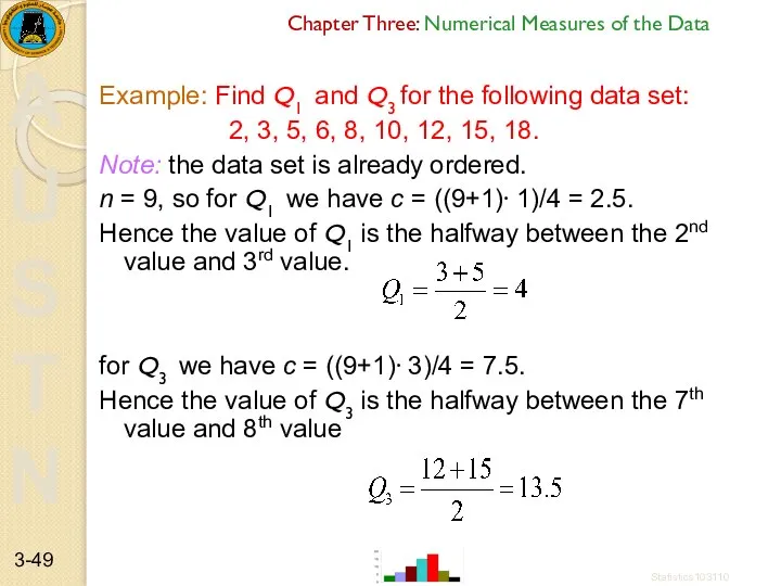
- 49. Chapter Three: Numerical Measures of the Data Example: Find Q1 and Q3 for the following data
- 50. Chapter Three: Numerical Measures of the Data Example: For the following data set: 2, 3, 5,
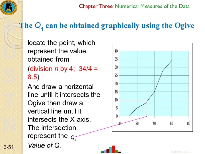
- 51. Chapter Three: Numerical Measures of the Data The Q1 can be obtained graphically using the Ogive
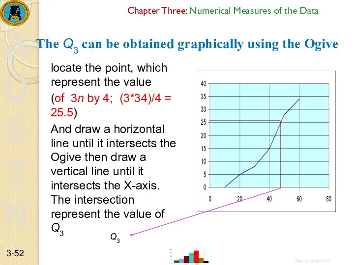
- 52. Chapter Three: Numerical Measures of the Data The Q3 can be obtained graphically using the Ogive
- 53. Chapter Three: Numerical Measures of the Data The Interquartile Range (IQR) The Interquartile Range, IQR =
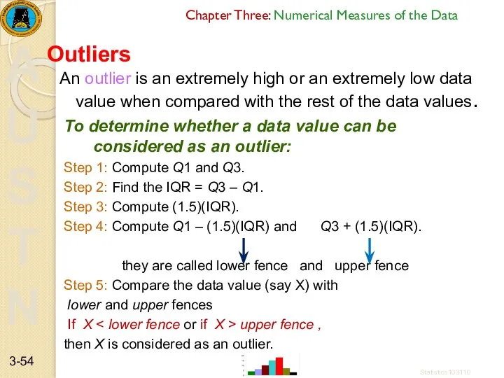
- 54. Chapter Three: Numerical Measures of the Data An outlier is an extremely high or an extremely
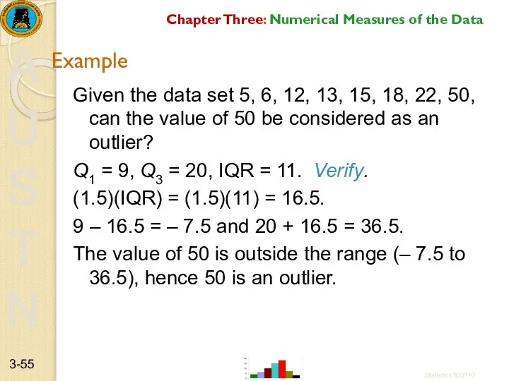
- 55. Example Given the data set 5, 6, 12, 13, 15, 18, 22, 50, can the value
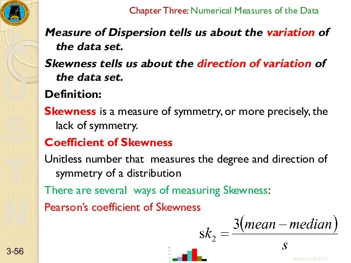
- 56. Chapter Three: Numerical Measures of the Data Measure of Dispersion tells us about the variation of
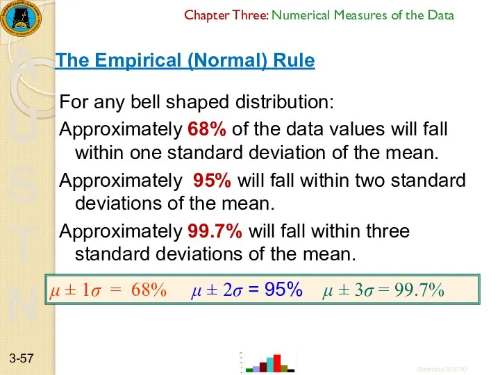
- 57. Chapter Three: Numerical Measures of the Data For any bell shaped distribution: Approximately 68% of the
- 58. The Empirical (Normal) Rule μ ± 1σ = 68% μ ± 2σ = 95% μ ±
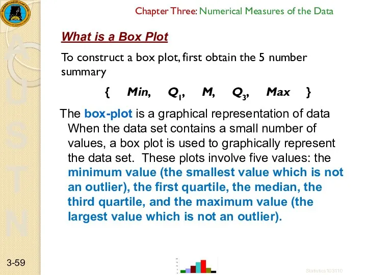
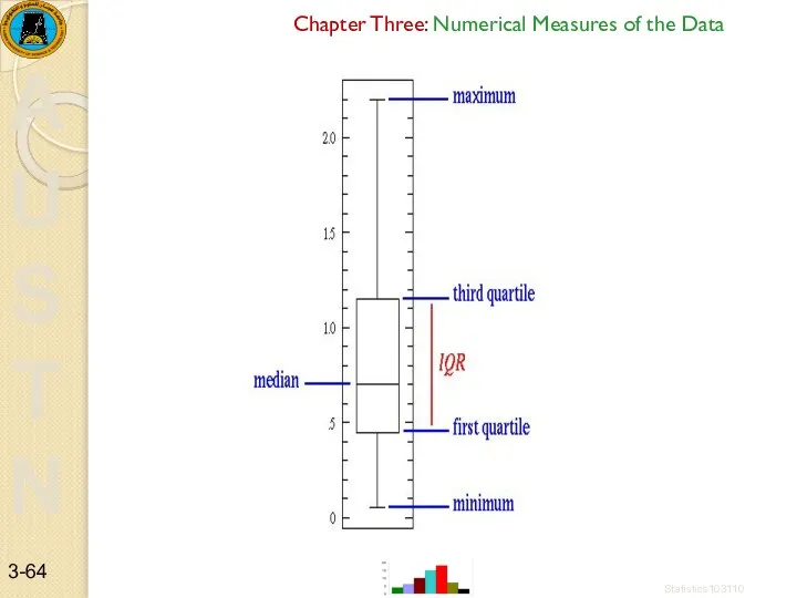
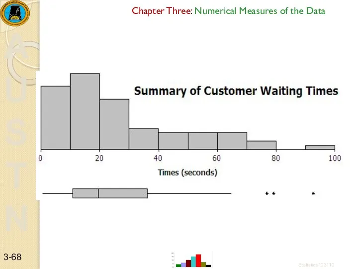
- 59. Chapter Three: Numerical Measures of the Data What is a Box Plot To construct a box
- 60. The box plot is useful in analyzing small data sets that do not lend themselves easily
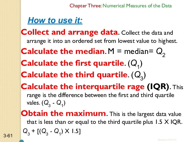
- 61. How to use it: Collect and arrange data. Collect the data and arrange it into an
- 62. Obtain the minimum. This value will be the smallest data value that is greater than or
- 63. Example 1:- Failure times of industrial machines (in hours) 32.56 42.02 47.26 50.25 59.03 60.17 61.56
- 64. Chapter Three: Numerical Measures of the Data Statistics103110 3-
- 65. Chapter Three: Numerical Measures of the Data Now find the interquartile range (IQR). The interquartile range
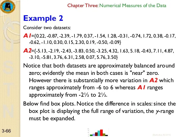
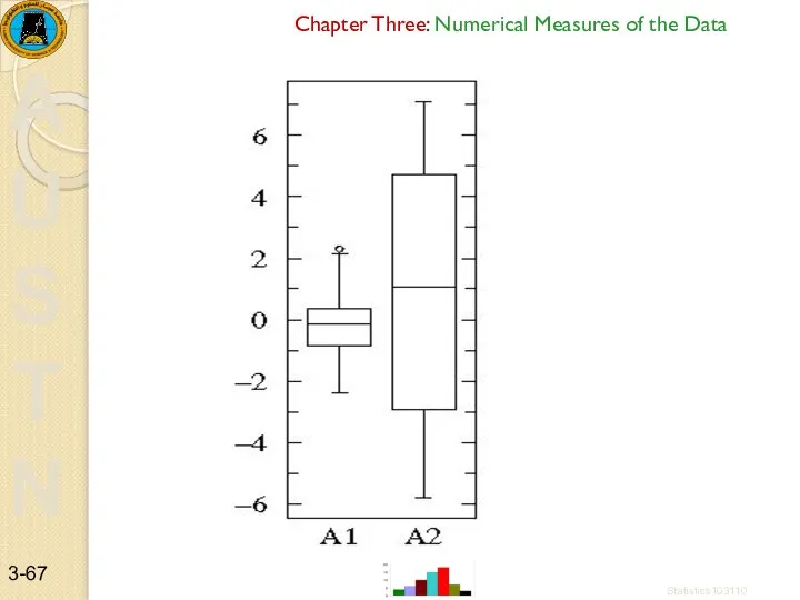
- 66. Chapter Three: Numerical Measures of the Data Example 2 Consider two datasets: A1={0.22, -0.87, -2.39, -1.79,
- 67. Chapter Three: Numerical Measures of the Data Statistics103110 3-
- 68. Chapter Three: Numerical Measures of the Data Statistics103110 3-
- 70. Скачать презентацию
Chapter Three: Numerical Measures of the Data
Outline
Introduction
3-1 Measures of Central Tendency
3-2
Chapter Three: Numerical Measures of the Data
Outline
Introduction
3-1 Measures of Central Tendency
3-2
Chapter Three: Numerical Measures of the Data
Objectives
Summarize data using the measures
Chapter Three: Numerical Measures of the Data
Objectives
Summarize data using the measures
Chapter Three: Numerical Measures of the Data
3-1 Measures of Central tendency
We
Chapter Three: Numerical Measures of the Data
3-1 Measures of Central tendency
We
Chapter Three: Numerical Measures of the Data
Example:- (Sample Mean)
The ages of
Chapter Three: Numerical Measures of the Data
Example:- (Sample Mean)
The ages of
Chapter Three: Numerical Measures of the Data
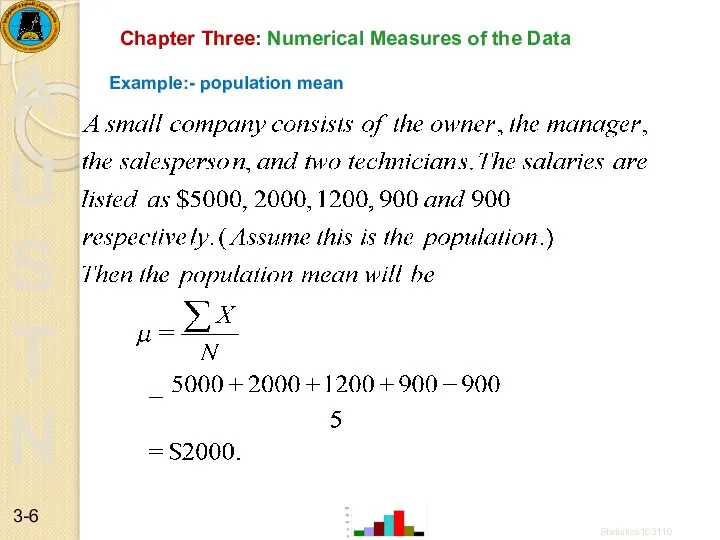
Example:- population mean
Statistics103110
3-
Chapter Three: Numerical Measures of the Data
Example:- population mean
Statistics103110
3-
Chapter Three: Numerical Measures of the Data
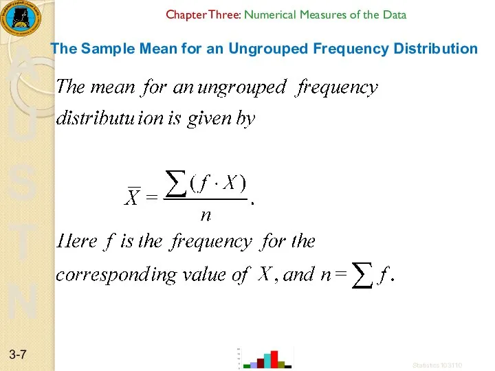
The Sample Mean for an
Chapter Three: Numerical Measures of the Data
The Sample Mean for an
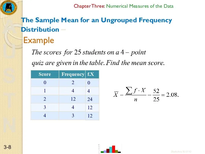
Chapter Three: Numerical Measures of the Data
The Sample Mean for an
Chapter Three: Numerical Measures of the Data
The Sample Mean for an
Chapter Three: Numerical Measures of the Data
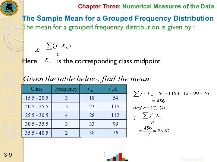
The Sample Mean for a
Chapter Three: Numerical Measures of the Data
The Sample Mean for a
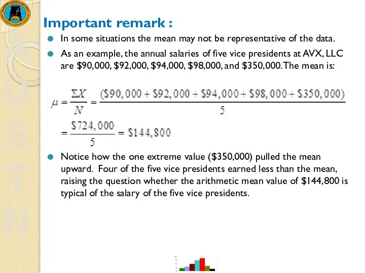
Important remark :
In some situations the mean may not be representative
Important remark :
In some situations the mean may not be representative
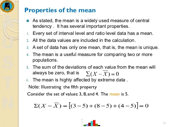
Properties of the mean
As stated, the mean is a widely
Properties of the mean
As stated, the mean is a widely
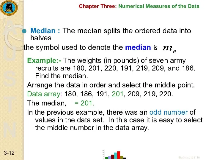
Chapter Three: Numerical Measures of the Data
Median : The median splits
Chapter Three: Numerical Measures of the Data
Median : The median splits
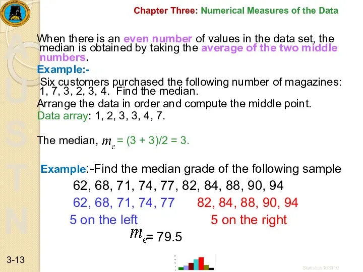
Chapter Three: Numerical Measures of the Data
When there is an even
Chapter Three: Numerical Measures of the Data
When there is an even
example
Find the median grade of the following sample of students grades
example
Find the median grade of the following sample of students grades
Properties of the Median
The major properties of the median are:
The median
Properties of the Median
The major properties of the median are:
The median
Chapter Three: Numerical Measures of the Data
Mode:- is the score that
Chapter Three: Numerical Measures of the Data
Mode:- is the score that
Chapter Three: Numerical Measures of the Data
Example:- Eleven different automobiles were
Chapter Three: Numerical Measures of the Data
Example:- Eleven different automobiles were
Chapter Three: Numerical Measures of the Data
The Mode for a Grouped
Chapter Three: Numerical Measures of the Data
The Mode for a Grouped
Properties of the Mode
The mode can be found for all levels
Properties of the Mode
The mode can be found for all levels
Chapter Three: Numerical Measures of the Data
The weighted mean is used
Chapter Three: Numerical Measures of the Data
The weighted mean is used
Chapter Three: Numerical Measures of the Data
Example:- During a one hour
Chapter Three: Numerical Measures of the Data
Example:- During a one hour
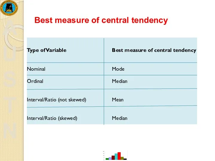
Best measure of central tendency
Best measure of central tendency
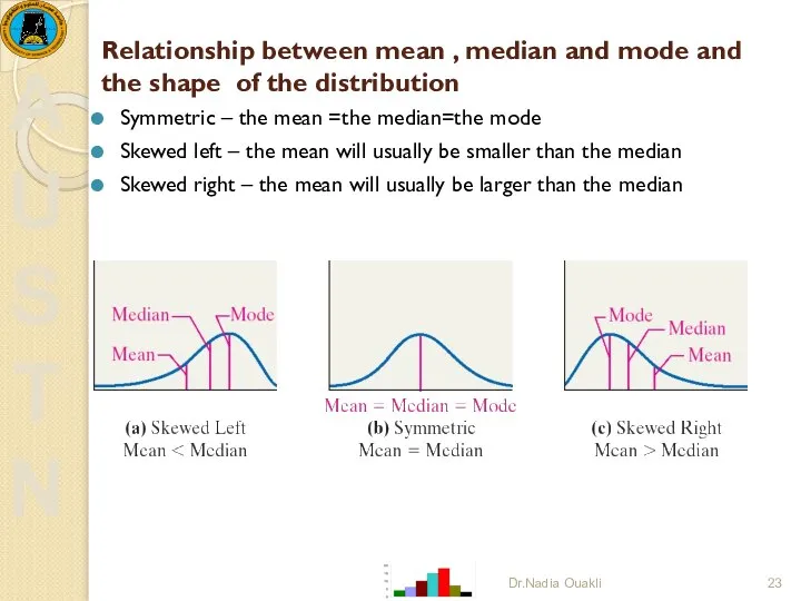
Relationship between mean , median and mode and the shape of
Relationship between mean , median and mode and the shape of
Chapter Three: Numerical Measures of the Data
3-2 Measures of Dispersion( variation)
o
Chapter Three: Numerical Measures of the Data
3-2 Measures of Dispersion( variation)
o
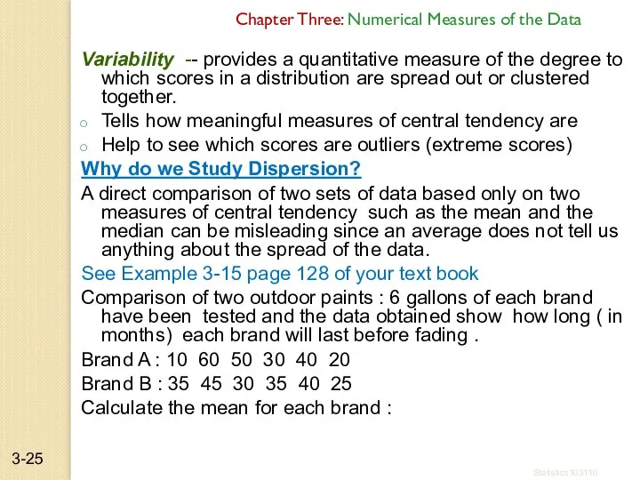
Variability -- provides a quantitative measure of the degree to which
Variability -- provides a quantitative measure of the degree to which
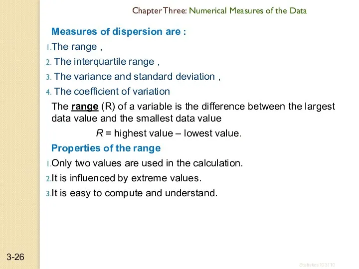
Measures of dispersion are :
The range ,
The interquartile range
Measures of dispersion are :
The range ,
The interquartile range
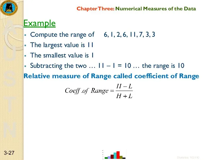
Example
Compute the range of 6, 1, 2, 6, 11, 7, 3,
Example
Compute the range of 6, 1, 2, 6, 11, 7, 3,
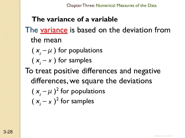
The variance of a variable
The variance is based on the deviation
The variance of a variable
The variance is based on the deviation
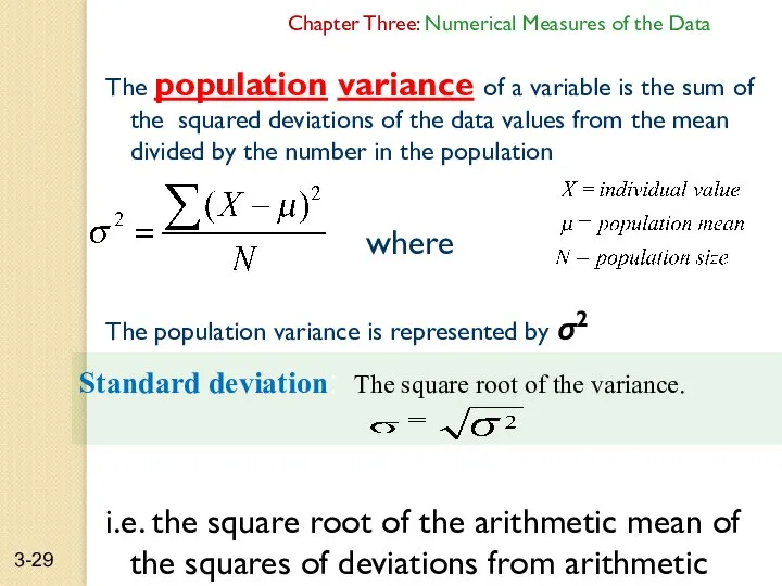
Chapter Three: Numerical Measures of the Data
The population variance of a
Chapter Three: Numerical Measures of the Data
The population variance of a
Properties of the variance and standard deviation
it is the typical or
Properties of the variance and standard deviation
it is the typical or
Chapter Three: Numerical Measures of the Data
The sample variance of a
Chapter Three: Numerical Measures of the Data
The sample variance of a
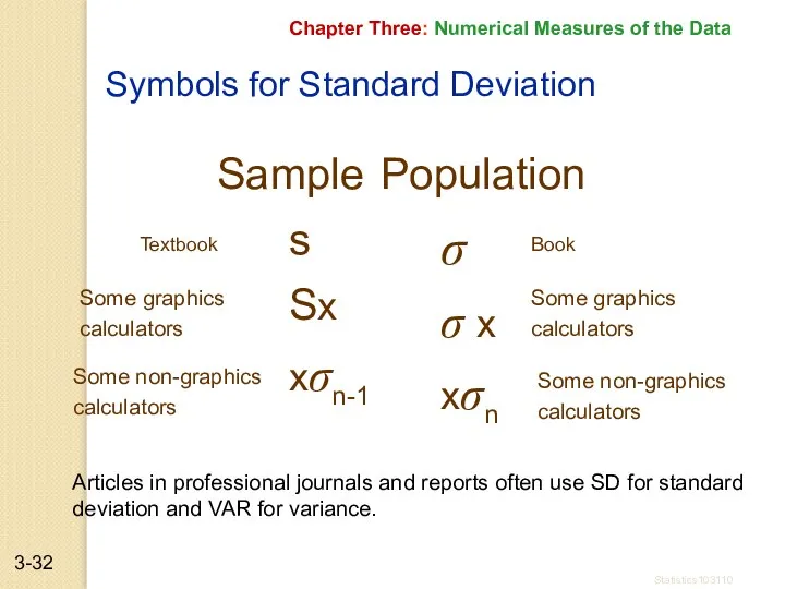
Symbols for Standard Deviation
Sample
Population
σ
σ x
xσn
Book
Some graphics
calculators
Some non-graphics
calculators
Textbook
Some graphics
calculators
Some non-graphics
calculators
Articles in
Symbols for Standard Deviation
Sample
Population
σ
σ x
xσn
Book
Some graphics
calculators
Some non-graphics
calculators
Textbook
Some graphics
calculators
Some non-graphics
calculators
Articles in
Chapter Three: Numerical Measures of the Data
Sample Variance for Grouped and
Chapter Three: Numerical Measures of the Data
Sample Variance for Grouped and
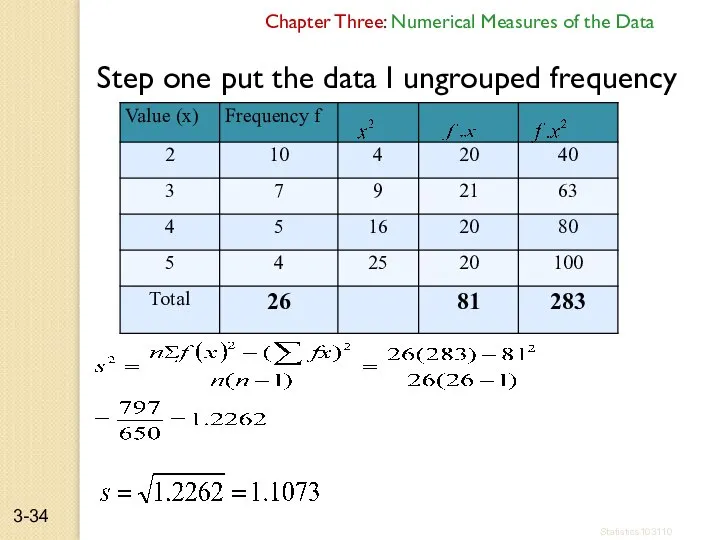
Step one put the data I ungrouped frequency table
Chapter Three: Numerical
Step one put the data I ungrouped frequency table
Chapter Three: Numerical
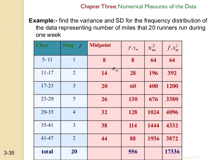
Example:- find the variance and SD for the frequency distribution of
Example:- find the variance and SD for the frequency distribution of
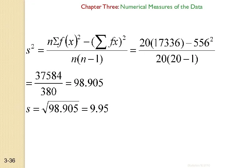
Chapter Three: Numerical Measures of the Data
Statistics103110
3-
Chapter Three: Numerical Measures of the Data
Statistics103110
3-
Chapter Three: Numerical Measures of the Data
Interpretation and Uses of the
Chapter Three: Numerical Measures of the Data
Interpretation and Uses of the
Chapter Three: Numerical Measures of the Data
Coefficient of Variation :-
The
Chapter Three: Numerical Measures of the Data
Coefficient of Variation :-
The
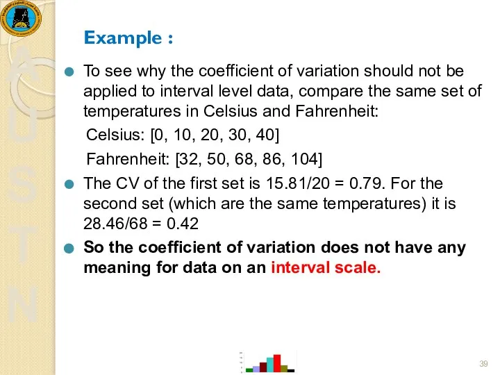
Example :
To see why the coefficient of variation should not be
Example :
To see why the coefficient of variation should not be
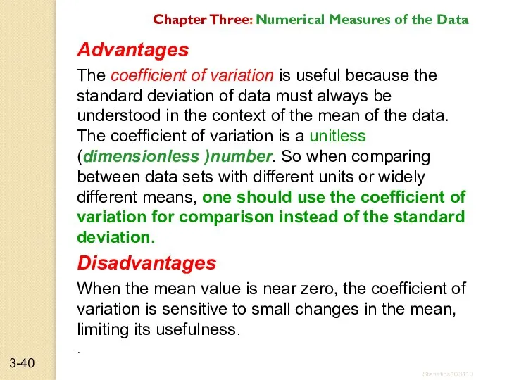
Advantages
The coefficient of variation is useful because the standard deviation of
Advantages
The coefficient of variation is useful because the standard deviation of
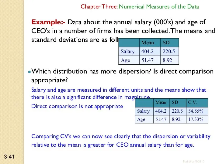
Example:- Data about the annual salary (000’s) and age of CEO’s
Example:- Data about the annual salary (000’s) and age of CEO’s
Chapter Three: Numerical Measures of the Data
Measure of position:
Measures of position
Chapter Three: Numerical Measures of the Data
Measure of position:
Measures of position
Chapter Three: Numerical Measures of the Data
Standard Scores (or z-scores) specify
Chapter Three: Numerical Measures of the Data
Standard Scores (or z-scores) specify
Chapter Three: Numerical Measures of the Data
Characteristics of Standard Scores
The shape
Chapter Three: Numerical Measures of the Data
Characteristics of Standard Scores
The shape
Chapter Three: Numerical Measures of the Data
Example:- A student scored 65
Chapter Three: Numerical Measures of the Data
Example:- A student scored 65
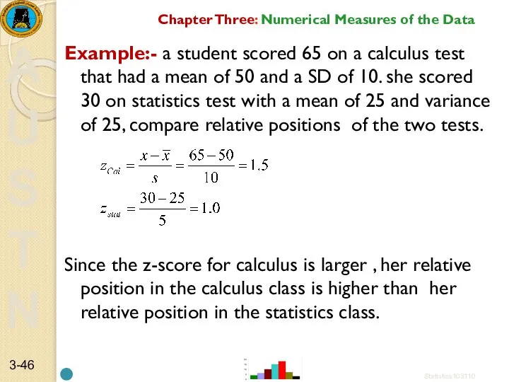
Example:- a student scored 65 on a calculus test that had
Example:- a student scored 65 on a calculus test that had
Chapter Three: Numerical Measures of the Data
Quartiles divide the data set
Chapter Three: Numerical Measures of the Data
Quartiles divide the data set
Chapter Three: Numerical Measures of the Data
Example:
For the following
Chapter Three: Numerical Measures of the Data
Example:
For the following
Chapter Three: Numerical Measures of the Data
Example: Find Q1 and Q3
Chapter Three: Numerical Measures of the Data
Example: Find Q1 and Q3
Chapter Three: Numerical Measures of the Data
Example:
For the following
Chapter Three: Numerical Measures of the Data
Example:
For the following
Chapter Three: Numerical Measures of the Data
The Q1 can be obtained
Chapter Three: Numerical Measures of the Data
The Q1 can be obtained
Chapter Three: Numerical Measures of the Data
The Q3 can be obtained
Chapter Three: Numerical Measures of the Data
The Q3 can be obtained
Chapter Three: Numerical Measures of the Data
The Interquartile Range (IQR)
The Interquartile
Chapter Three: Numerical Measures of the Data
The Interquartile Range (IQR)
The Interquartile
Chapter Three: Numerical Measures of the Data
An outlier is an extremely
Chapter Three: Numerical Measures of the Data
An outlier is an extremely
Example
Given the data set 5, 6, 12, 13, 15, 18, 22,
Example
Given the data set 5, 6, 12, 13, 15, 18, 22,
Chapter Three: Numerical Measures of the Data
Measure of Dispersion tells us
Chapter Three: Numerical Measures of the Data
Measure of Dispersion tells us
Chapter Three: Numerical Measures of the Data
For any bell shaped distribution:
Approximately
Chapter Three: Numerical Measures of the Data
For any bell shaped distribution:
Approximately
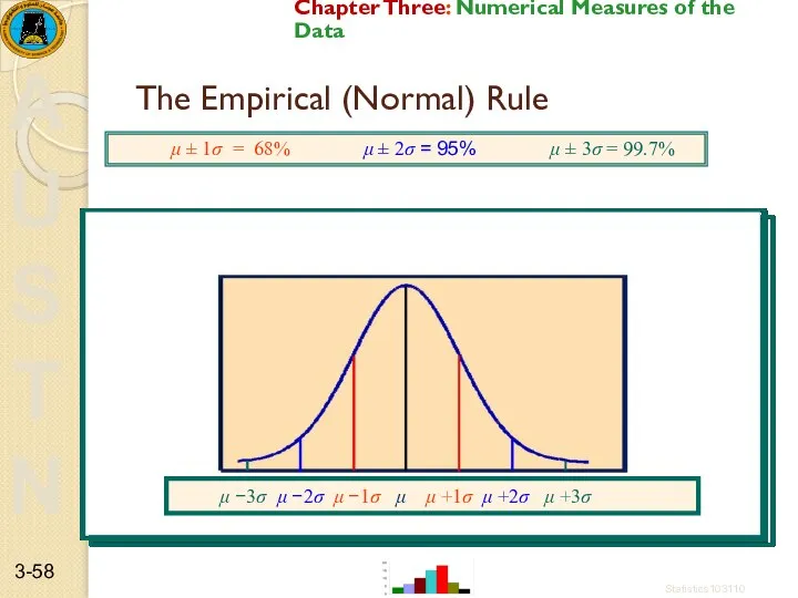
The Empirical (Normal) Rule
μ ± 1σ = 68% μ ±
The Empirical (Normal) Rule
μ ± 1σ = 68% μ ±
Chapter Three: Numerical Measures of the Data
What is a Box Plot
Chapter Three: Numerical Measures of the Data
What is a Box Plot
The box plot is useful in analyzing small data sets that
The box plot is useful in analyzing small data sets that
How to use it:
Collect and arrange data. Collect the data and
How to use it:
Collect and arrange data. Collect the data and
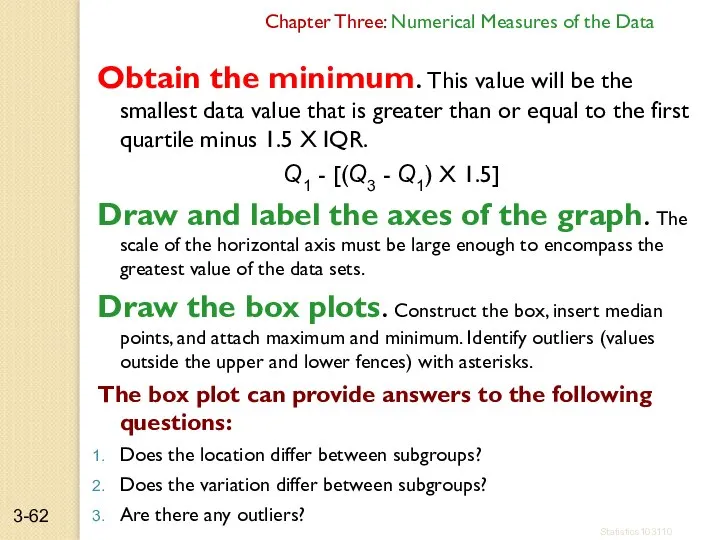
Obtain the minimum. This value will be the smallest data value
Obtain the minimum. This value will be the smallest data value
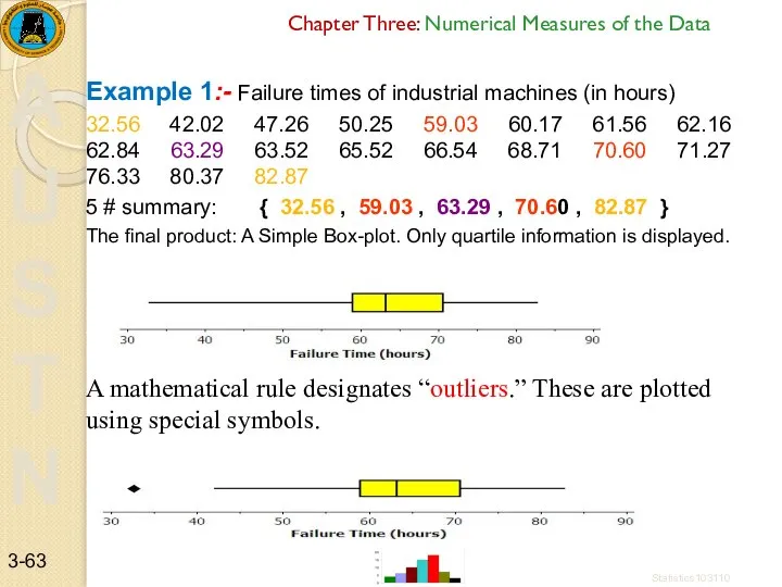
Example 1:- Failure times of industrial machines (in hours)
32.56 42.02 47.26
Example 1:- Failure times of industrial machines (in hours)
32.56 42.02 47.26
Chapter Three: Numerical Measures of the Data
Statistics103110
3-
Chapter Three: Numerical Measures of the Data
Statistics103110
3-

Chapter Three: Numerical Measures of the Data
Now find the interquartile range (IQR). The
Chapter Three: Numerical Measures of the Data
Now find the interquartile range (IQR). The
Chapter Three: Numerical Measures of the Data
Example 2
Consider two datasets:
A1={0.22, -0.87,
Chapter Three: Numerical Measures of the Data
Example 2
Consider two datasets:
A1={0.22, -0.87,
Chapter Three: Numerical Measures of the Data
Statistics103110
3-
Chapter Three: Numerical Measures of the Data
Statistics103110
3-
Chapter Three: Numerical Measures of the Data
Statistics103110
3-
Chapter Three: Numerical Measures of the Data
Statistics103110
3-
 Величины и их измерение. (Тема 4)
 Число и цифра 4
 Аттестационная работа. Организация познавательной деятельности на уроках математики в 5 классе
 Статистические критерии различий (3). Критерии различий. Сравнение более двух выборок
 Презентация по математике "Теория бесконечных множеств. Часть 2" - скачать бесплатно
 Что? Где? Когда? Математическая игра
 Подготовка к контр работе. Решение задач по теме: площади. Теорема Пифагора.(первый урок)
 Таблица умножения. Тренажер
 Сумма углов в треугольнике
 Основы математического моделирования
 Умножение и деление положительных и отрицательных чисел. Урок 48
 Презентация по математике "Системы счисления. Задачи" - скачать
  Формулы. Решение задач
 Единицы массы: грамм, килограмм
 Презентация по математике "Координаты на поле" - скачать
  Открытый урок в 10 «В» классе на тему: «Тригонометрические уравнения»
 Анықталмағандықтар. Лопиталь ережес
 Применение производной к исследованию функций
 Дифференциальное исчисление функций нескольких переменных
 Задачи на построение
 Интерактивные тренинги по математике для подготовки к ЕГЭ
 Подготовка к контрольной работе №5. Свойства прямоугольного треугольника
 Связь между суммой и слагаемыми
 Модели статистического прогнозирования (11класс)
 Процент төшенчәсе белән танышу. Процентлар табу
 Расстояние от точки до плоскости. Теорема о трех перпендикулярах
 Квадратичная функция, её свойства и график
 Теорема Пифагора