- Forecasting. Successful operations of the company

Содержание
- 2. Successful operations of the company Effective planning Accurate forecasting
- 3. Forecasting techniques: Mechanical extrapolation Simulation Linear interpolation Exponential smoothing Barometric methods Leading indicators Compound indexes Diffuse
- 4. Mechanical extrapolation Forecasting techniques Originally extrapolation methods are mechanical and not closely linked to economic theory
- 5. However, they are widely used by professional economists who make forecasting Because of they are easy
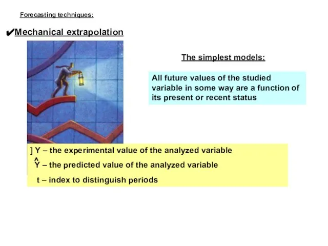
- 6. Mechanical extrapolation The simplest models: All future values of the studied variable in some way are
- 7. Mechanical extrapolation Forecasting techniques: The simplest models: Unchanging model The predicted value of the variable for
- 8. The vast majority of all economic, political and social decisions are made based on considered the
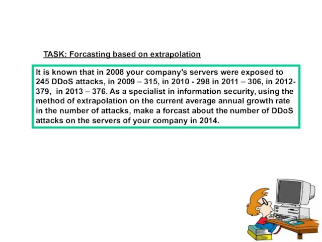
- 9. TASK: Forcasting based on extrapolation It is known that in 2008 your company's servers were exposed
- 10. 2. The average annual growth rate is an indicator of the intensity changes in the levels
- 11. 3. Chain growth rate is the ratio of each next level of series to previous and
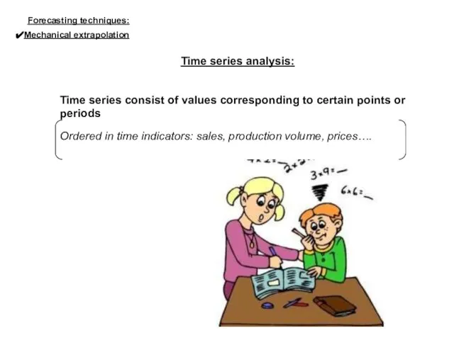
- 12. Time series analysis: Time series consist of values corresponding to certain points or periods Ordered in
- 13. Why fluctuation is typical for the time series? Usually there are four sources of variation in
- 14. 1) Trend (Т) Is a long-term increase or decrease of series Seasonal changes (S) Due to
- 15. 3) Cyclic changes (С) Cover periods of several years, reflect the level of economic boom or
- 16. Seasonal changes and the method of moving average Moving average is calculated by summing the values
- 17. Regroup presented data: Time series analysis: Mechanical extrapolation Forecasting techniques: Using the data presented in the
- 18. Step 1: Moving average over the four periods is calculated using a consistent set of sales
- 19. Step 5: Make normatization: the average value of the four average seasonal indexes must be equal
- 20. Q1: 316 (для 1989) * 0,99 = 312,84 $ Q2: 322 (для 1989) * 1,38 =
- 21. Designing of trend As a forecasting method assumes that started change in the variable will continue
- 22. ] Y – the observed value of the analyzed variable Y – the predicted value of
- 23. Trend estimates are more reliable if they are based on data released from seasonal effects Seasonal
- 24. Y = 284,382 + 1,632 t Year centralized moving Average Y Period total
- 26. Скачать презентацию
Successful operations of the company
Effective planning
Accurate forecasting
Successful operations of the company
Effective planning
Accurate forecasting
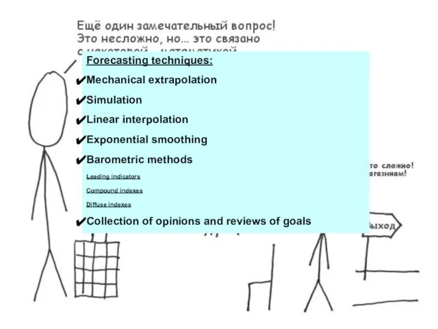
Forecasting techniques:
Mechanical extrapolation
Simulation
Linear interpolation
Exponential smoothing
Barometric methods
Leading
Forecasting techniques:
Mechanical extrapolation
Simulation
Linear interpolation
Exponential smoothing
Barometric methods
Leading

Mechanical extrapolation
Forecasting techniques
Originally extrapolation methods are mechanical
and not closely linked to
Mechanical extrapolation
Forecasting techniques
Originally extrapolation methods are mechanical
and not closely linked to

However, they are widely used by professional economists who make forecasting
Because
However, they are widely used by professional economists who make forecasting
Because
Mechanical extrapolation
The simplest models:
All future values of the studied variable in
Mechanical extrapolation
The simplest models:
All future values of the studied variable in

Mechanical extrapolation
Forecasting techniques:
The simplest models:
Unchanging model
The predicted value of the
Mechanical extrapolation
Forecasting techniques:
The simplest models:
Unchanging model
The predicted value of the
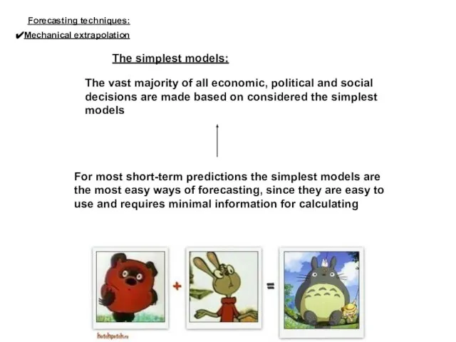
The vast majority of all economic, political and social decisions are
The vast majority of all economic, political and social decisions are
TASK: Forcasting based on extrapolation
It is known that in 2008 your
TASK: Forcasting based on extrapolation
It is known that in 2008 your
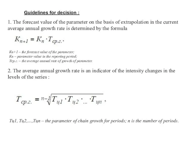
2. The average annual growth rate is an indicator of the
2. The average annual growth rate is an indicator of the
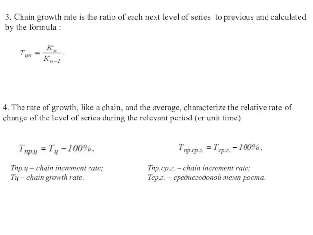
3. Chain growth rate is the ratio of each next level
3. Chain growth rate is the ratio of each next level
Time series analysis:
Time series consist of values corresponding to certain points
Time series analysis:
Time series consist of values corresponding to certain points
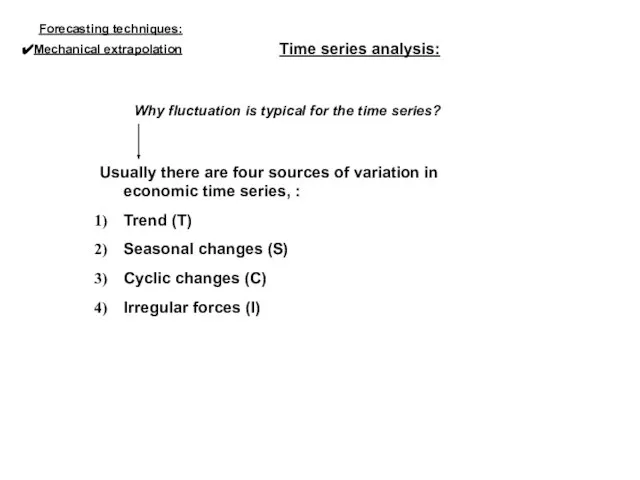
Why fluctuation is typical for the time series?
Usually there are four
Why fluctuation is typical for the time series?
Usually there are four
1) Trend (Т)
Is a long-term increase or decrease of series
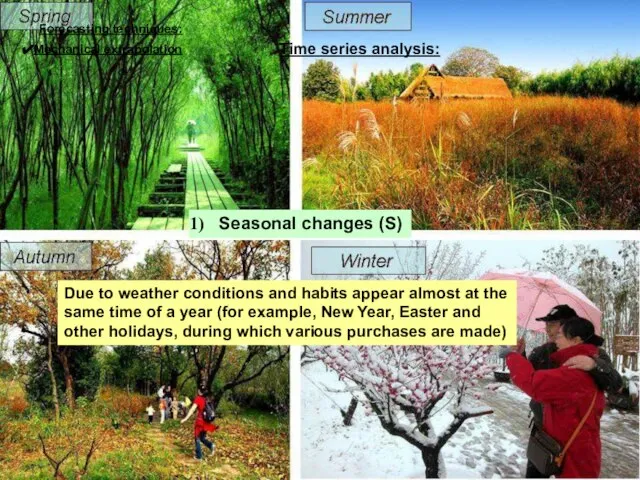
Seasonal changes
1) Trend (Т)
Is a long-term increase or decrease of series
Seasonal changes
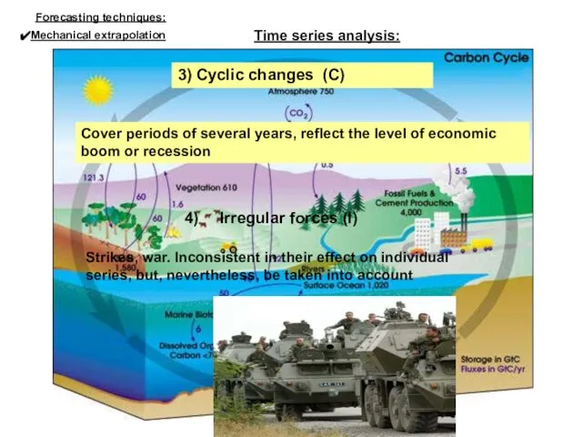
3) Cyclic changes (С)
Cover periods of several years, reflect the level
3) Cyclic changes (С)
Cover periods of several years, reflect the level
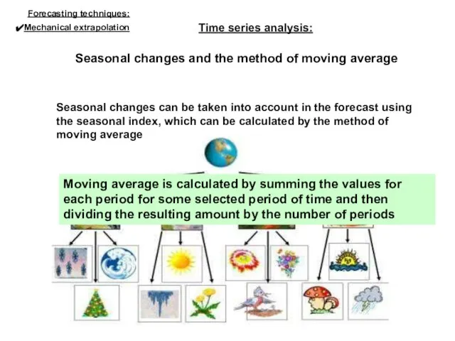
Seasonal changes and the method of moving average
Moving average is calculated
Seasonal changes and the method of moving average
Moving average is calculated

Regroup presented data:
Time series analysis:
Mechanical extrapolation
Forecasting techniques:
Using the data presented in
Regroup presented data:
Time series analysis:
Mechanical extrapolation
Forecasting techniques:
Using the data presented in
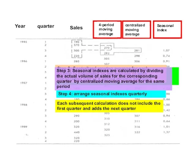
Step 1: Moving average over the four periods is calculated using
Step 1: Moving average over the four periods is calculated using
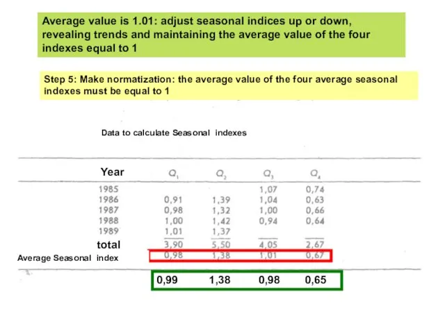
Step 5: Make normatization: the average value of the four average
Step 5: Make normatization: the average value of the four average

Q1: 316 (для 1989) * 0,99 = 312,84 $
Q2: 322 (для
Q1: 316 (для 1989) * 0,99 = 312,84 $
Q2: 322 (для

Designing of trend
As a forecasting method assumes that started change in
Designing of trend
As a forecasting method assumes that started change in
![] Y – the observed value of the analyzed variable Y](/_ipx/f_webp&q_80&fit_contain&s_1440x1080/imagesDir/jpg/587663/slide-21.jpg)
] Y – the observed value of the analyzed variable
Y
] Y – the observed value of the analyzed variable
Y
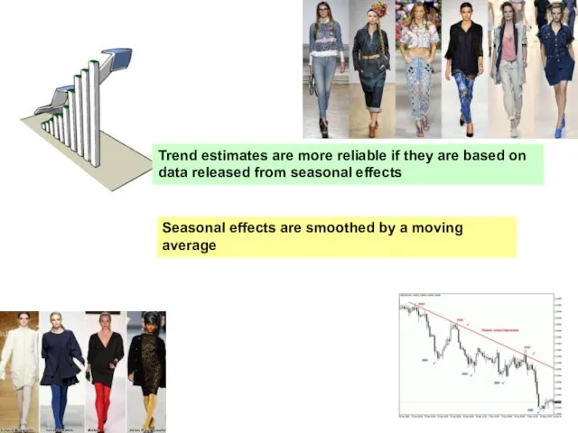
Trend estimates are more reliable if they are based on data
Trend estimates are more reliable if they are based on data
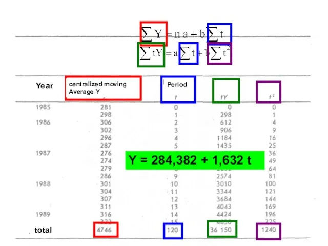
Y = 284,382 + 1,632 t
Year
centralized moving Average Y
Period
total
Y = 284,382 + 1,632 t
Year
centralized moving Average Y
Period
total
 Разработка методов и моделей доставки тарно-штучных грузов из Юго-Восточной Азии в Россию
 Стратегическое управление эффективностью бизнеса ОАО ФосАгро
 Діагностика виникнення і розвитку кризового процесу в туризмі
 Принципы работы в команде
 Теоретические основы управления изменениями
 Совершенствование логистической деятельности производственного предприятия
 Мероприятия по стимулированию продаж
 Управление качеством и сертификация услуг общественного питания. Тема 1
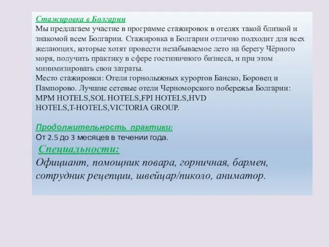 Стажировка в Болгарии
 Менеджер по работе с поставщиками
 Организация как система управления
 Содержание предпринимательской деятельности
 Концепции управления запасами
 Управление человеческими ресурсами
 Транспортно-экспедиционная компания ТЭК Росавтотранс Сарапул
 Управление магазином подарков. Урок №11
 Общая характеристика менеджмента
 Управление методическим и психологическим сопровождением инноваций в образовательном процессе
 Роль этического менеджмента в современной организации
 Менеджменттің пайда болуы
 Менеджмент в образовании
 Деловые коммуникации
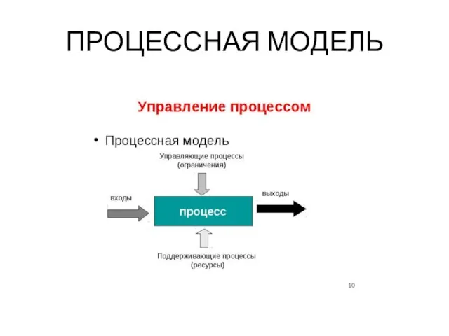 Процессная модель
 Транспортная система Agam Vergus, приложение TransEgmoVargus
 Work-life balance подход в управлении рабочим временем молодых сотрудников
 Участие в организации производственной деятельности в рамках структурного подразделения деревообрабатывающего производства
 Функции менеджмента: контроль и координация
 Что должен знать руководитель о мотивации сотрудников